Chapter 1 Toss up: coin flips

The simplest kind of statistical experiment involves flipping coins to detect if the coin is fair: equally likely to turn up heads or tails. Many statistics texts start here. Although my goal is to upend statistical pedagogy with this book, I’ll start here too. One reason, besides convention, is that my preferred, simulation-based approach, is simple to describe and execute in this setting. It makes for a nice warm-up. We can do the entire analysis without any fancy math. Now, connecting to what other textbooks and software libraries provide does require math, and we won’t shy away from that in this book. But I’ll kick that can down the road a little bit to later chapters, beginning in Chapter 3.

It’s amazing what you can do with a computer and a simple R program. This is true for coin flipping experiments, as described here, but also for much more involved scenarios. Convincing you of that is one of the goals of this book. Giving you the tools and intuition required to do it, and connecting you to results and nomenclature involved in a more conventional analysis, is another. If you’ve taken a university-level course in statistics (or perhaps a high-school level advanced placement class), then you may have heard the term “null hypothesis”. This concept is very important to statistical inquiry. Perhaps because it helps make a connection to the scientific method where the formulation and (usually) rejection of hypotheses play a central role. Statistical methods are often involved in the advance of science.

Yet students find hypothetical formalism off-putting. Consequently, I don’t like it, especially not as pertains to an early introduction of an otherwise digestible subject for someone who is quantitatively inclined. Like you, I hope. So I poke fun at it with my title, “null hippopotamus” (or hipp0 for short). I prefer to instead ponder, “what if’s”. So that’s how we’ll start.

I’ll bring some of the formalism in too, so that connections can be made to convention. I don’t want to hang you out to dry when it comes to communicating with others, and understanding analysis in the literature. Throughout, my goal is to keep it simple. That doesn’t mean there won’t be rigor. Yet the focus will be more squarely on statistical ideas, and on the intuition that they provide through data. I’m no pedant for scientific vocabulary.

Alright, enough disclaimer. Suppose your buddy flipped a coin thirty times, and this was the outcome, where H means “heads” and T means “tails”.

data <- c("H", "T", "H", "H", "H", "T", "T", "H", "T", "T", "H", "H", "H",
  "T", "T", "H", "H", "H", "H", "T", "H", "H", "H", "T", "H", "H", "T", 
  "H", "T", "T")

And now you want to know: is the coin fair? You’re not allowed to inspect the coin, flip the coin more times, nothing. All you’ve got from your buddy is the outcome of those thirty flips. Those are your data. Your observations.

1.1 Simulation

But that doesn’t mean you can’t bring something of your own to the table. You could always flip a different coin – one you know to be fair – and compare what you get to the data. I know what you’re thinking. Why would I do that when I already know what the outcome would be? I’d get about the same number of heads as tails, right? Wrong. That’s the thing about chance. Anything could happen. You could flip that fair coin thirty times and get all heads, or all tails, or you could alternate heads, tails, etc., fifteen times, and all other things in between. Some such events are rare. A run of all heads has probability $1/2^{30}$, which is about one in 10 billion. But, if everyone in the world did it, then chances are one person would get “lucky”. (At the time of writing, there are 8 billion souls on Earth.)

This isn’t a book on probability. I’ll assume you have some experience, and quickly review relevant concepts as necessary, often pointing to Wikipedia, like I did above for several key vocabulary words. This book, and perhaps you might say the enterprise of statistical inquiry more generally, is about combining probability with data to draw conclusions about how things (might) work. It’s a deep subject, but many of its tenets are simple, and many basic recipes are both intuitive and work well.

Ok, so suppose we flip our own coin thirty times. Let’s not actually do that with a real coin, because that’s super monotonous. Instead, let’s get our computer to do it for us. There are a lot of ways to do this. For example, each flip could go like this:

u <- runif(1)   ## generate single pseudo-random number uniformly in [0,1]
f <- "T"
if(u >= 0.5) f <- "H"
f

## [1] "T"

The outcome is random and may be different when you try it on your own. It certainly will if you do it over and over again, and I encourage you to do that. I’m not going to explain how pseudo-random number generators work, but I will note that most use a uniform $[0,1]$ generator, or $u \sim \mathcal{U}[0,1]$, as a building block, or subroutine, just like I did above. Notice how I converted $u \geq 1/2$ into “heads”, and otherwise “tails”.

A more streamlined way to do that in R would be to use the binomial generator, rbinom.

c("T", "H")[rbinom(1, 1, 0.5) + 1]

## [1] "H"

Again, the outcome is random and I encourage you to repeat that (many times) and see what you get. The output of rbinom(1, 1, 0.5) is either 0 or 1. You can read up on it with ?rbinom in R, but here are the highlights that are relevant for now. A call to rbinom(n, x, p) will “flip a coin” x times with probability (1 - p, p) of (0, 1), respectively, record the sum of those flips, and repeat that n times and report all the sums. Under the hood, it uses runif. You can download the source code from https://cran.r-project.org if you’re curious and see how it all works. So if you provide n=1 and x=1, it’s basically the same as a coin flip, but with outcome of 0 or 1 rather than heads or tails. My code above makes the conversion from binary to characters “T” or “H”.

Quick digression on terminology. Flipping (weighted) coins is known formally as sampling from a Bernoulli distribution. We’ll talk in more detail about that later. I capitalized Bernoulli because it’s named after a Swiss mathematician. A binomial distribution is the sum of repeated Bernoulli trials, or flips. I just wanted to tell you that so you could understand where the function name rbinom comes from. We’ll come back to the binomial distribution later too.

Alright, back to flipping coins. Adjusting the n argument to rbinom gets you more flips of a single coin.

sim <- c("T", "H")[rbinom(30, 1, 0.5) + 1]
sim

##  [1] "H" "T" "T" "H" "H" "H" "H" "T" "T" "T" "T" "H" "T" "T" "T" "H"
## [17] "H" "H" "H" "H" "T" "T" "T" "T" "T" "H" "T" "H" "T" "T"

You get a similar outcome by holding fixed n=1 and adjusting x=30, but this is a little more complex since it requires a vector p argument. Perhaps tinker with that on your own if you’re curious.

Ok, now we have thirty flips that come from a fair coin and thirty that come from our buddy who may or may not have used a fair coin. What do we do? It makes sense to somehow compare them to one another, but there are lots of ways we could do that. I’m sure you have a way in mind – probably the same as mine – but just to convince you there are others, I’ll list a few silly ones.

Look at each pair of first flips and see if they’re the same.
Look at each pair of second flips, third, etc.
Measure the length of the longest “run” of consecutive tails (or heads) for each.
Measure the length of the second longest “run” for each.
Measure the length of the longest alternating “T”, then “H” run for each.

And so on like that. These are pretty bonkers, admittedly, but none of them is a wrong choice. Some of them are quantitatively inferior to others, in a way that will take a little while to explain in more detail.

For now, it stands to reason that if you only look at the first flip, or the second flip, then you’re not being very efficient about things because you’re not using all of the collected information. That inefficiency will likely lead to the wrong conclusion just by chance. Moreover, if you only pair your first flip with your buddy’s first flip, or second with second, then you’re artificially imposing an order to otherwise probabilistically independent events. That’s not ideal either.

A sensible choice, and likely the one you’re thinking of, is to count the number of heads (or equivalently tails) separately for both sets of thirty flips. In code …

Hd <- sum(data == "H")
Hs <- sum(sim == "H")
c(buddy=Hd, sim=Hs)

## buddy   sim 
##    18    13

Any numerical summary of data, like the sensible one above but also the silly ones earlier, is called a statistic. Intuitively, the best statistics summarize the data with the fewest quantities possible without losing any relevant information. I’ll make this more specific later. For now, counting the number of heads is pretty good on this account since knowing that number, along with the total number of flips (30), tells you just about everything from the experiment. You can deduce from that the number of tails (30 minus the count of heads). With those two numbers, you know about the outcome of the entire experiment, except the order in which the flips came in. But if we regard flips as independent, order doesn’t really matter. None of the other silly statistics above let you do that.

We actually have two statistics. One summarizes the observational data (Hd), where some aspect of the data-generating mechanism is unknown to us/beyond our control, and about which we desire to make an inference. (Is the coin fair?) The other comes from a simulation (Hs) where we know the “coin” was fair. Both are subject to randomness: the data from the chaotic dynamics of coin flipping, and the simulation from pseudo-random numbers. These are not the same thing, so we acknowledge that by saying that the simulated data are from, or a realization of, a model for actual coin flips. We could have chosen a more elaborate model, perhaps one based on the physics of coin tossing (Stefan and Cheche 2016), but that’s for a different book.

Keeping it simple for now, let’s presume our simulation is a decent stand-in for the actual data-generating mechanism. No model is perfect, but this one seems good enough to be useful. Our simulated and observed statistics are not equal, and together they tell a strange story. We expect fifteen heads in a sample of thirty when the coin is fair. When we knew the coin was fair, in our simulation, we got 13 (less than that). The data, where we don’t know if the coin was fair, gave us 18 (more than that). What gives? How is any of this helpful?

We now have a sense of the inherent randomness in the problem: the spread of what could happen when flipping thirty coins. To take things to the next level, we must flip even more (sets of thirty) coins. I know, strange right? If doing it once is perplexing, how could doing it even more times make things better, not worse? Hold that thought for a moment. Before I show you what to do, and how it works and why, I’ll need to invest in a little notation. What I’m about to show you works for pretty much everything, not just flipping coins. In a way, the entire book is here in the first chapter. The rest of the book is just practice appropriating the idea for other scenarios.

1.2 Notation and nomenclature

You might not like it, but it’s helpful here to make a brief digression and invest in some mathematical notation. This will help make things concrete and generic at the same time. That in a nutshell, I think, encapsulates the investment in mathematical reasoning. It begins by making a simple thing, like coin flips, harder and possibly inscrutable to the uninitiated. But then you gain some familiarity through experience and value emerges. The additional sophistication that thoughtful mathematical notation and reasoning provides not only makes things look more elegant, but also allows us to be much more specific about the calculations involved. Don’t worry, there isn’t much math required for the time being.

The letter I prefer for random experimental outcomes (i.e., observations) – and preferred in most statistical circles, whether that be mainstream stats, machine learning and artificial intelligence, or data science more broadly – is $y$. We capitalize $Y$ to refer to a random, as yet unknown outcome (like for a coin flip). We would say that $Y$ is a random variable, which is explicitly or implicitly endowed with some probabilistic distribution that prescribes the chances that it could take on particular values, once observed.

Quick digression on $Y$. You might say, “we used $X$ in my other stats class.” That may be, and $X$ is good too, but $Y$ is better because of regression (Chapters 7, 12 and 13). Take my word for it. If you’re tempted to substitute $X$ everywhere I use $Y$, please don’t. You’ll regret it. Suspend disbelief and force yourself to learn a new way. You’ll be smarter for it. $X$ will come back later.

Alright, back to random variables. Particular values random $Y$ could take on are notated in lowercase, like $y$. Lowercase is also used to refer to values already observed (say, in data). For example, we could refer to $\mathbb{P}(Y = y)$, which is the probability of observing that random variable $Y$ takes on value $y$. We can refer to the outcome of a random event or experiment that hasn’t happened yet as $Y$, or one that has already (and we’ve seen the outcome) as $y$.

In the case of flipping coins, the convention is to notate $y = 1$ for heads and $y = 0$ for tails. That way, we can introduce a parameter $\theta$ that controls the rate of heads and describe the distribution as follows:

\[\begin{equation} \mathbb{P}(Y = y) = f(y; \theta) = \theta^y (1- \theta)^{1-y}, \quad \theta \in [0,1], \tag{1.1} \end{equation}\]

where $f(y; \theta)$ could generically stand in for any probability density (pdf) or mass function (pmf), but above a Bernoulli mass is used for binary data. Check that under this setup $f(1; \theta) = \theta$ and $f(0; \theta) = 1-\theta$, which means that the probability of heads is $\theta$ and one minus that for tails, as it should. In our experiment we wondered if the coin is fair, and that scenario corresponds to $\theta = 0.5$.

Quick digression on lettering. If you follow the link to the Bernoulli distribution on Wikipedia, you’ll see that the letter $p$ is used instead of $\theta$. This is non-standard in most statistical circles where Greek letters are preferred for parameters. Roman letters are for data quantities. Parameters are unknown quantities that must be estimated from data. So I think of parameters as ideals we’ll aspire to learn but never achieve exactly. We shall never ascend to enlightenment (think lofty Greek gods and philosophers), but with data we can dial in estimates and move things along from a practical perspective (think practical Roman imperialism, though they also had their gods). I will follow this throughout in the book.

Alright, back to coins. Mass $f(y; \theta)$ is for just one coin. What about thirty coins? The letter that’s usually used in statistics for a number of experimental trials, or number of data points, is $n$. There are $n=30$ in our coin flipping experiment. This is a good point to convert our code from §1.1 to use this new notation. I always find it helpful when object names, which are called symbols in computer programming vernacular, match up with math (the names of the variables) as much as possible.

y <- as.numeric(data == "H")
n <- length(y)
Ys <- as.numeric(sim == "H")

Operator == creates what in R is called a logical vector, composed of TRUE and FALSE values. I encourage you to try that part separately, before as.numeric which coverts Boolean values to zeros and ones.

Note that y and Ys are n-length vectors, not scalars. They hold observed data values $y_1, \dots, y_n$ and simulated versions, respectively. Instead of Y for simulated values, as an analog of random variable $Y$, I prefer Ys. There are a number of reasons. One is that simulated Ys holds not unknown, random, values but actual ones I generated. Another is that I like to remind myself that they came from a simulation. So the name I prefer for the symbol is a compromise between the notion it represents and the manner in which the values were generated. A final thing worth mentioning is that the code above for Ys is basically yielding what rbinom(30, 1, 0.5) does, when we first generated sim above, before mapping those values to "H" and "T".

For experiments like this, it’s common to make the assumption that experimental units – each coin flip – are independent of one another and that they follow the same probabilistic (Bernoulli) distribution. In other words, they are independent and identically distributed, abbreviated as iid (usually written in lowercase). The first “i” in iid, for independence, means that the joint probability of all $n$ observations (flips) factorizes as the product of the probability of the individual ones. Recall that, by definition, two events $A$ and $B$ are independent if

\[ \mathbb{P}(A,B) = \mathbb{P}(A) \mathbb{P}(B). \]

That may be extended, by repeated application, to all $n$ events ($n=30$ coin flips) as follows.

\[\begin{equation} \mathbb{P}(Y_1 = y_1, \dots, Y_n = y_n) \stackrel{\mathrm{iid}}{=} \prod_{i=1}^n \mathbb{P}(Y_i = y_i) \tag{1.2} \end{equation}\]

If they are also identically distributed, the second “id” in iid, then $\mathbb{P}(Y_i = y_i) = f(y_i; \theta)$. In other words, each $Y_i$ has the same mass or density function $f$, and with identical parameter $\theta$, for all $i=1,\dots,n$. In the case of a Bernoulli (1.1), it would be common to write the statistical model out in shorthand as follows.

\[ \mbox{Model:} \quad \quad Y_i \stackrel{\mathrm{iid}}{\sim} \mathrm{Bern}(\theta), \quad i=1,\dots, n \]

Check in this setup that

\[\begin{equation} \mathbb{P}(Y_1 = y_1, \dots, Y_n = y_n) = \theta^{\sum y_i} (1- \theta)^{n - \sum y_i}, \tag{1.3} \end{equation}\]

where $\sum y_i \equiv \sum_{i=1}^n y_i$. Dropping the bounds is a common shorthand especially when sums reside in powers.

Notice that $\sum y_i$, which is the same as the number of heads in our $n$ flips, is an important statistic. We came across this quantity by intuition earlier, and now it has some mathematical justification. I see this as a bonus. There’s nothing wrong with intuition as the basis for deciding on something. It also doesn’t hurt to have mathematical reasoning to point to, especially if someone doubts your intuitive chops. We’ll revisit this in much more detail later. In general, a statistic $s_n = s(y_1, \dots, y_n)$ is some function that summarizes your data. Often it distills $n$ quantities down to one scalar, but not always.

Now let’s circle back to the specific coin flipping problem, collect thoughts, and codify what we have and what we want to know in mathematical terms. We have $n=30$ flips, summarized by the count of the number of heads $s_{30} = 18$. Again, endowing our code with the new symbols …

s <- sum(y)           ## observed statistic
Ss <- sum(Ys)         ## simulated statistic
c(s=s, Ss=Ss, n=n)

##  s Ss  n 
## 18 13 30

Nothing has really changed; these are just new names for things in code to match the math.

Now, I want to know if the coin is fair ($\theta = 0.5$) or not ($\theta \ne 0.5$). The statistical, mathematical way to describe this “want to know” is through the following formal hypotheses:

\[\begin{align} \mathcal{H}_0 &: \theta = \textstyle \frac{1}{2} && \mbox{null hypothesis (``what if'')} \tag{1.4} \\ \mathcal{H}_1 &: \theta \ne \textstyle\frac{1}{2} && \mbox{alternative hypothesis.} \notag \end{align}\]

The way that we use evidence, which comes from observed data via our statistic $s_n$, is by making a contradiction argument. Assume the opposite of what the data is telling you, that the null hypothesis $\mathcal{H}_0$ is true even though you didn’t get what you expected, and see where that leads compared to quantities actually calculated from observed data. Or, you can think about it as “innocent until proven guilty”. The simpler, null hypothesis corresponds to the accused being innocent of a crime. It is up to a prosecutor to convince a jury that something more complicated, more nefarious, is in play.

It’s hard to carry two imperfect metaphors through to fruition at once, so bear with me. Here’s what we’ve got. For fair coin flips we might expect $s_n = \sum_{i=1}^n y_i = n/2$, or 15 for 30 flips.² So $\mathcal{H}_0$ is the “what if”. And if it turns out this null hypothesis is false, you should be able to propagate that, logically speaking, to some blatant mathematical contradiction. Carrying this out, and coming to a conclusion, is what is meant by a statistical hypothesis test.

It’s worth remarking that it’s certainly possible that we could get $s_n = 15$ for any $\theta$, fair coin or no. The opposite is also true: even with $\theta = 0.5$ we could observe $s_n \ne 15$, and we did when we simulated coin flips in §1.1. But usually the null hypothesis/“what if” is a simplifying choice of convenience – something favoring parsimony – rather than something we generally believe to be true.

For example, having every/any minted coin be exactly fair is preposterous. Surely it must be that each coin slightly favors heads or tails in the long run, due to manufacturing irregularities. Yet as long as quality control at the mint is relatively high, we probably wouldn’t have the patience to flip the coin enough times to tell. So a sensible baseline “what if” is that the coin is fair, versus the alternative that it is not. For an actually (or close to) fair coin a prosecutor will need a lot of evidence – a lot of flips – to tell. But for our friend’s particular coin, which maybe was purchased at a magic shoppe, a good lawyer may be able to build a case with fewer.

Algorithm 1.1: “Want to know what if” (or, testing statistical hypotheses)

Assume you have some data $y_1,\dots, y_n$ and a statistical model caricaturing the data generating mechanism.

Require complementary null ($\mathcal{H}_0$) and alternative ($\mathcal{H}_1$) hypotheses encoding what you want to know, and a statistic $s_n = s(y_1, \dots, y_n)$ that you can calculate from your data.

Then

Pretend $\mathcal{H}_0$ is true (your “what if”) and under those conditions (i.e., with your model), calculate or derive the sampling distribution of $S_n = s(Y_1,\dots, Y_n)$.
Compare the observed statistic $s_n$ to the distribution of $S_n$.
- If $s_n$ looks typical under $S_n$, then $\mathcal{H}_0$ is probably reasonable (“fail to reject $\mathcal{H}_0$”);
- otherwise, “reject” $\mathcal{H}_0$ in favor of the alternative $H_1$.

Report your conclusions/evidence.

Enough mixing of metaphors. The actual procedure is outlined in Alg. 1.1. It’s framed generically, because it has nothing to do with coin flips. The idea is to have something to circle back to later, and over and over again. Notice what is “assumed” and “required”, which are both things that the practitioner must provide, in a sense. You need some data, obviously, and you pair that with a probabilistic model for how the data is generated. That model will likely have some (unknown) parameters, like $\theta$, but may not always.

Then, the practitioner must specify what he or she “wants to know” in terms of competing hypotheses. These are usually opposites of one another. The null one ($\mathcal{H}_0$) is simpler or more constrained, in some sense, than the alternative ($\mathcal{H}_1$) which represents the unconstrained version. Often these have to do with a parameter $\theta$, but again not always. For example, Eq. (1.4) contrasts $\theta = 0.5$ with $\theta \ne 0.5$, and these are complements of one another.

Finally, the practitioner needs to choose a statistic, $s_n = s(y_1,\dots, y_n)$ which provides the wedge that (potentially) forms evidence for an alternative against the null. Like in a trial by jury, a prosecutor must present specific evidence that distills a complex situation (lots of data) down to a few things $s_n$ (DNA from blood on a knife) to focus scrutiny. Whoops, I used a metaphor again. Sometimes $s_n$ is referred to as a test statistic because it is a statistic that is used to conduct a hypothesis test.

The precise relationship between null and alternative hypotheses, and what it means about the procedure and the interpretation of its outcome, is subtle and we’ll get into more detail on that later. The real stars of the show, for now and in great generality, are the observed data, model, null hypothesis $\mathcal{H}_0$ and statistic $s_n$. These are in bold in Alg. 1.1; you must have these four ingredients before you can get started.

The null describes how observed data could be generated under the chosen probabilistic model, comprising our “what if” in Step 1. Those choices can be parlayed into a distribution over possible values of the statistic $S_n$. This is known as the sampling distribution of the statistic. It is also known as the null distribution, making a direct link to $\mathcal{H}_0$ involved in a statistical test. All statistical tests involve comparing the observed value of the statistic, $s_n$, calculated on the actual data, to the distribution of possible values $S_n$ under the null.

$S_n$ under $\mathcal{H}_0$ (with the model) is a random variable, which is why it is capitalized. $Y_1, \dots, Y_n$ values that could arise in the “what if” scenario that $\mathcal{H}_0$ is true yields $S_n = s(Y_1, \dots, Y_n)$. A function $s(\cdot)$ of random variables $Y$ is itself a random variable $S$. Note that I’m using subscripts a little differently for $Y$ and $y$ than for $S$ and $s$. For $Y$-values the subscript indicates the sample record number, or index into a vector. For $S$, which is often a scalar but almost always of smaller dimension than the sample size $n$, subscript $n$ is intended to remind you of how many data points the statistic is calculated from.

In old fashioned statistics, you would use math – sometimes a lot of fancy advanced math that’s way over my head – to derive the form of the sampling distribution of $S_n$ under $\mathcal{H}_0$. We’ll see some of that later. When the math is doable, I’ll do it. When it’s not, I’ll show you where to look. Perhaps one of the most important deliverables of this book, however, is that you don’t need fancy math if you have a computer.

Before we transition to that, let me address the hippopotamus in the room. What? I think that the use of the term “hypothesis” in statistics is awkward. We don’t really believe that any of this stuff is “true”, null or alternative. I already said that we don’t believe that coin flips come from a Bernoulli distribution. Because they don’t. So it’s a bit harebrained to hypothesize that they do. Yet the Bernoulli is a useful simplifying assumption, because it makes things concrete probabilistically. And anyways, all models are wrong.

I already said I think we use the word hypothesis in statistics in order to connect with tenets of the scientific method. That’s a noble enterprise. Also, scientists seem to have a fetish for Greek words, like algorithm and logarithm, which (sorry!) there will be a lot of in this book.³

This book is about statistical evidence and procedures like Alg. 1.1 that try to adjudicate between one option or another for how observational data we have in hand could have arisen. For that, I prefer the simpler, less snooty, plain English “want to know” or “what if”. I want to know: could data generated in a certain way have given rise to statistics that are similar to what I observed from actual data? The way I do that is to see “what (happens) if” synthetic data are generated that way, and then make a comparison. That comparison can happen via the sampling distribution, and that’s what we’ll do next.

So if, like me, you don’t like the word hypothesis, just substitute it with hippopotamus. If you’re not advanced enough to do the hard math that’s sometimes needed to derive the sampling distribution, I’ll show how you can do it by Monte Carlo sampling from $\mathcal{H}_0$. In other words, “Monty the null hippopotamus”. That’s easy to remember, and easy to do.

1.3 Monte Carlo

Here I focus on Steps 1–2 of Alg. 1.1 by returning to the simulation idea from §1.1, but doing it a lot! In other words, we build up an understanding of the sampling distribution of a statistic under the null hypothesis by sampling from that distribution. That sounds vacuous, and therefore potentially meaningless, but perhaps that’s because as a notion it’s so simple. And after you see what I mean, because we’re going to do it momentarily, (I hope) you’ll think “oh yeah, that’s obvious and easy to do” on a computer. And, in the case of flipping coins, you could even do it without a computer but it would be a bit tedious.

People used to do stuff like this without a computer. To understand the chances that certain random occurrences would/could happen, they would repeatedly try them over and over again and keep a tally of the number of times they got various outcomes. Nowhere is this more widely understood, and perhaps more important to operations, than with games of chance that involve money. I mean gambling in casinos. Those casinos want to make sure that they make money – to make sure the house wins on aggregate – so they invest a lot of resources into understanding the odds. Then they try to pair those odds with payouts that seem lucrative for the client, to entice them to play, but also ensure profitability not only in the long run, but also in the worst case.

One of the most prominent modern-day gambling spots, and home to some of the oldest casinos that are still in operation today, is Monte Carlo, Monaco. Monte Carlo is a strange and fascinating place, and I encourage you to read more about it. There are casinos there that have been open since the 19th century. Back in the day, they didn’t have computers to help visualize things and make it cheap to explore odds. So they would play the games of chance over and over again and keep tabs. That’s what we’re going to do here, but on a computer.

Although we’ll use Monte Carlo (MC) sampling primarily for statistical purposes, the Monte Carlo method has broad applicability in mathematical calculations with computers, most notably integration. In fact, there is a sense that what we’re doing here is basically an integral – I mean from calculus – but we’ll talk more about that later. For now, let’s just see how it works for entertaining “what if’s”.

Alright, head back to §1.1 where we simulated $n=30$ coin flips and compared those to observed data. We converted those to $y$- and $s$-values in §1.2. And now we’re going do that lots more times, comprising a MC simulation experiment. Without further ado, the code below gathers $N=10,000$ samples of the test statistic under $\mathcal{H}_0$ by repeatedly flipping fair coins $Y_1, \dots, Y_n$ and calculating $S_n$ for those values by summing them up.

N <- 10000                        ## number of MC "trials"
Ss <- rep(NA, N)                  ## storage for sampled test statistics
for(i in 1:N) {                   ## each MC trial
  Ys <- rbinom(n, 1, 0.5)         ## generate n (=30) virtual coin flips
  Ss[i] <- sum(Ys)                ## calculate the test statistic
}

Notice how each sample of the statistic in the vector Ss is saved, but not all of the $N \times n$ coin flips. Once we’ve summed them up, we don’t need the flips anymore.

Ok, now what to do with that? There are many ways to inspect samples from a distribution. My favorite generally, and the best for our purposes here, is a histogram. Figure 1.1 provides that visual, overlayed with some additional information that I shall discuss momentarily. A histogram provides one way of visually inspecting empirical distribution, which basically means that its form depends on all of the numerical values in the data (in this case samples of $S_n$), rather than some summary of them or a (possibly estimated) parameter. So you could say that the histogram of Figure 1.1 comprises an empirical sampling distribution.⁴ More on empirical distributions, if you’re curious, is in §A.1. But I’m hoping you can get the gist with experience.

hist(Ss, main="") 
abline(v=c(s, n-s), lty=1:2, col=2, lwd=2)
legend("topright", c("s", "reflect"), col=2, lty=1:2, lwd=2, bty="n")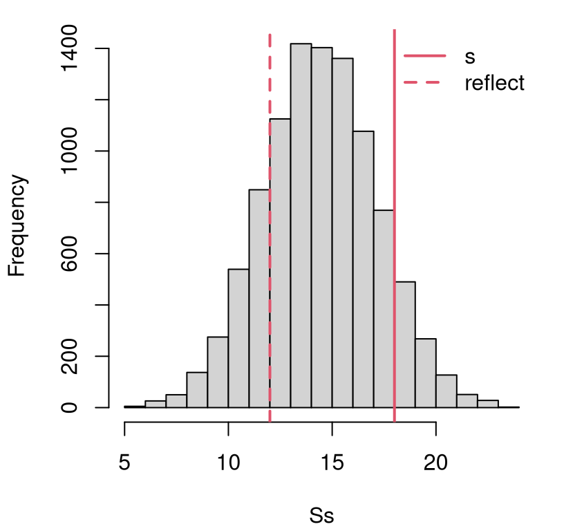

$Histogram of samples $S_n$ from the sampling distribution under $\mathcal{H}_0$, and the actual $s_n$ (and it’s “two-tailed” reflection) for comparison, for the coin flipping experiment.$

FIGURE 1.1: Histogram of samples $S_n$ from the sampling distribution under $\mathcal{H}_0$, and the actual $s_n$ (and it’s “two-tailed” reflection) for comparison, for the coin flipping experiment.

The vertical red lines in the figure are particularly important as they represent different views on the value of the statistic $s_n$ calculated from observed coin flip data. The position of the solid one is exactly at $s_n$ on the $x$-axis. For me, its position indicates that the value of $s_n$ we observed from actual data is not atypical under the sampling distribution for $S_n$ derived from the null hypothesis.

Flipping a fair coin $n= 30$ times gives rise to $s_{30} = 18$ heads regularly, and even more (extreme) counts. That’s not a rare occurrence at all! Therefore, I can’t “reject” the hypothetical “what if” that the actual observational data $y_1, \dots, y_n$ could have been generated from conditions described by the assumed (Bernoulli model) data generating mechanism under $\mathcal{H}_0$. I must be willing to accept that the null hypothesis may be true.

Quick digression on terminology here. Alg. 1.1 says that, in this case, I should “fail to reject $\mathcal{H}_0$”, but I said “willing to accept”. Many instructors would take off points for such blasphemy. Not me. You can say whatever you want in my book. I sure will. You can read many opinions online, like this one, asserting that acceptance “implies that the null hypothesis is by nature true, and it is proved”. Poppycock! That’s not how the word “accept” is used in the English language. I don’t know how people used it in the 19th century, when stats was in its early days. Today people “accept” an idea when they don’t want to quibble. They want the conversation to keep moving. It’s a matter of politeness, not conviction or gospel truth. I’m not going to quibble with you. I’m cool if you accept when you mean you weren’t able to reject, given the evidence in the data.

Remember, this modeling framework is all a convenient cartoon. Nothing in real life boils down to coin flips, not even coin flips. It’s a simplifying abstraction. There is no true, mathematical specification of the data generating mechanism. The null is never “by nature” anything, let alone true or false. Acknowledging that, we might choose to reject every $\mathcal{H}_0$ without even looking at the data. That’s not helpful. So when we fail to reject in our simplified, cartoon land, I’m ok with accepting however you want to tell me that.

Alright, back off my high horse. That’s basically it. Yet, anything important bears repeating. We sampled a statistic via synthetic data from the null distribution. If the actual observed version of the statistic looks typical (as it does in Figure 1.1) then we cannot reject the notion that $\mathcal{H}_0$ is true. If, rather, it looks rare or extreme, then we reject $\mathcal{H}_0$ in favor of the alternative $\mathcal{H}_1$, about which I shall say more momentarily.

Statisticians don’t like to rely purely on visuals, because “looking” lacks precision, and is beholden to human judgment which can be whimsical. They’d rather have hard figures. You can probably imagine many reasonable ways of quantifying the sentiment that an observed $s_n$ “looks typical or not” under the null distribution for $S_n$. Statisticians prefer to do that by calculating the probability of observing a more extreme $s_n$ under $\mathcal{H}_0$, where “more extreme” means toward the nearest tail (in the direction away from the mean) of the null distribution.

Such a quantity is easy to calculate with samples. We have $N = 10{,}000$ of them. Some are out in that tail (bigger than $s_n$), and some aren’t. That proportion (how many bigger over how many total) is approximating a probability that statisticians call a $p$-value. As $N\rightarrow \infty$ that proportion becomes exact for the $p$-value.

pval <- mean(Ss >= s)   ## same as sum(Ss >= s)/N, or (count/total)
pval

## [1] 0.1735

Something that happens 17% of the time isn’t rare at all. For historical reasons that are ultimately arbitrary and not of much interest to me (and thus to this book), statisticians have converged on a significance level of 5% as the threshold delimiting rare from typical. If the $p$-value is not less than 5%, then we can’t reject the null. I shall stick with that in this book and not give it much more thought. This value is sometimes written as $\alpha = 0.05$, suggesting one could choose another $\alpha$-value if they wanted to.

This $\alpha$ controls what is known as Type I error, which is pretty inscrutable as terminology goes. Basically, $\alpha$ controls the probability that you incorrectly reject $\mathcal{H}_0$. If you estimate $p \approx \alpha$, then you’ll be wrong $(100 \times \alpha)$% of the time. This presumes that all the other assumptions you’ve made, like about the statistical model generating the data, are true. (And we know they’re not.)

I wanted you to be aware of $\alpha$ and Type I error, but this book isn’t really about those details. Now that I’ve dispensed with them, I won’t bring them up again. I promise. But statisticians do another funny thing that I do need to tell you about, because it addresses an issue I brushed off earlier in §1.2 and promised to come back to: the alternative hypothesis $\mathcal{H}_1$. I’ll preface by saying that I find some of the logic here pretty unsatisfying, and easy to take issue with. Yet it’s not totally without sense and forms the basis of another important convention. Conventions are good because they let you get on with things by leveling the playing field. So we’ve gotta talk about it.

Our alternative hypothesis (1.4) was $\mathcal{H}_1: \theta \ne 0.5$, which means that the coin could be biased in either direction: more heads with $\theta > 0.5$ or more tails with $\theta < 0.5$. Our $p$-value calculation only focused on the “greater” side of the sampling distribution when evaluating the chances of seeing a more extreme statistic under $\mathcal{H}_0$. Looking only in the right tail corresponds to one-tailed or one-sided test.

Being biased either way ($\theta \ne 0.5$) allows for more wiggle room to accept the null – less likely to reject it – because the alternative is less specific. We saw more heads than would be expected under the null, but it just as easily could have been more tails. Performing a similar calculation on the other side of the sampling distribution provides the other tail. This is the meaning of the dashed vertical red line in Figure 1.1, which has been “reflected” into the left tail. Its value corresponds to n - s heads or s tails.

Combining one-tailed $p$-values, by adding together that of the original statistic and its reflection, yields a two-tailed test appropriate for an alternative hypothesis like $\mathcal{H}_1: \theta \ne 0.5$. The reflected one is hypothetical, representing the other tail.

pvals <- c(right=mean(Ss >= s), left=mean(Ss <= n - s),
       both=mean(Ss >= s) + mean(Ss <= n - s))
pvals

##  right   left   both 
## 0.1735 0.1881 0.3616

Note that the two-tailed $p$-value above is very similar, but not identical to, two times the one-tailed calculation. Sometimes you’ll see this described in textbooks, or on Wikipedia.

2*mean(Ss >= s)

## [1] 0.347

This does not give the same $p$-value because our sampling distribution is discrete, asymmetric, and composed of (way) fewer than $N$ unique values.

length(unique(Ss))

## [1] 20

There are only so many unique sums of $n$ coin flips – at most $n$ – but some, like with very few heads or tails, are highly improbable. In many situations, the two calculations agree (as $N \rightarrow \infty$), although the notion of a “reflection” is more nuanced, as we shall see later. This is just something to be aware of for now. Either way you calculate it, the two-sided $p$-value is larger than the one-sided one, so we still cannot reject $\mathcal{H}_0$.

Many statistical texts make a big deal about one- and two-sided tests, especially in homework exercises. A fair bit of the challenge in those problems involves sussing out which tail should be scrutinized. (A hint for working on problems like that: if your one-tailed $p$-value is bigger than $\frac{1}{2}$, then you’re probably working in the wrong tail.) I’m not going to give you those exercises here. This is not that kind of textbook. I want you to internalize the idea behind tests, and how you can do them in many settings through MC simulation. Figuring out whether you want a one- or two-tailed test is not really a statistical topic in my opinion.

All tests in this book will be two-sided by default. You can usually work out the one-sided version by eliminating the reflection. There are many tests, however, where there is no two-tailed test that makes sense. We’ll talk more about that when we get to it.

1.4 Wrapping up

Believe it or not, that’s it! Now you know how to do a hypothesis test for coin flips, or any binary/Boolean data from a Bernoulli process. You’ll have a chance to get some practice with homework problems in §1.5.

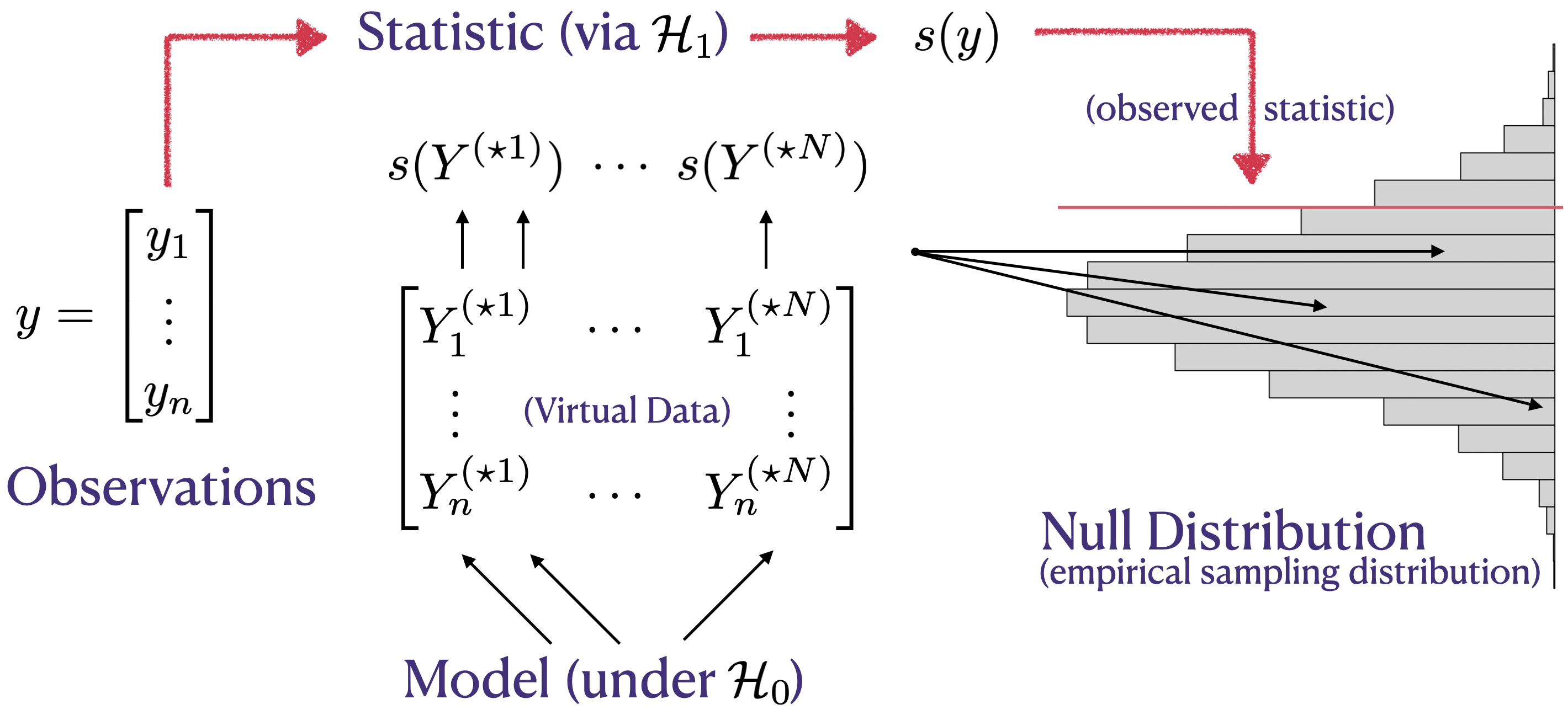
Hypothesis testing as a flow chart, capturing the relationship between key ingredients – data (observations), model, hypotheses, statistic – and the sampling distribution, represented via histogram.

FIGURE 1.2: Hypothesis testing as a flow chart, capturing the relationship between key ingredients – data (observations), model, hypotheses, statistic – and the sampling distribution, represented via histogram.

I made a little diagram that I hope will help augment the formal description in Alg. 1.1. See Figure 1.2. The diagram borrows a histogram representation of the (empirical) sampling distribution from the coin-flipping example, turned on its side in order to limit crossing of lines. So the diagram favors a MC adaptation of Alg. 1.1, but otherwise the flow is the same. The story behind the diagram, viewing it from left to right, goes like this.

You have some data $y$ and something you want to know about it. You must choose a probabilistic model for that data (e.g., coin flips with probability $\theta$ of heads), and frame your “want to know” as competing hypotheses. The null hypothesis ($\mathcal{H}_0$), the simpler or more restrictive of the two hypotheses, along with the model, informs the simulation. The model is used to generate virtual data, $Y^{(\star \cdot)}$ in the figure, or Ys in the code. The alternative hypothesis ($\mathcal{H}_1$) is more complex, providing evidence against the null, which may be helpful in determining an appropriate testing statistic $s(\cdot)$. Those two things combine to form the sampling distribution, allowing a comparison to be made between observed and simulated statistics. Details, like how to draw that comparison quantitatively, are ancillary. One way to do that is with a $p$-value.

I bet you can figure out how to adapt this to other settings on your own. To help, I’ll flesh out a lot of the details in later chapters. Eventually, we’ll need to invest in some higher-powered mathematics. There are two reasons for this. One is to help automate the choice of statistic $s_n$, which may be the single most important ingredient. The other is so that you can appreciate how my preferred MC approach compares to the old-school way of doing things, which is what most software packages provide. That comparison is not merely for culture. It’s important to relate to others, and see where strengths, weaknesses, and opportunities for synergy are. An old-school approach is complementary and has merits. And if you already have some experience doing things that way, I hope that this book will teach you a new – and I think highly transferable – skill.

Speaking of software. Suppose we wanted to encapsulate our work so we can use it later, for data from a different coin-flipping experiment. (Say, for your homework.) I mean a function that automates everything. Wrap it all up in a neat little bow. It might look something like monty.bern, below, where you can specify any $\theta \in [0,1]$.

### monty.bern:
###
### calculate a two-sided Bernoulli test via Monte Carlo and return 
### a p-value, along with optional visual
###
### s: test statistic from ...
### n: coin flips
### theta: null hypothesis proportion
### N: Monte Carlo effort
### vis: optional visualization
###
### uses auxiliary pval.discrete function provided on book webpage

source("pval_discrete.R")  ## details in Appendix B

monty.bern <- function(s, n, theta=0.5, N=10000, vis=FALSE)
{
  ## sanity checks
  if(length(s) != 1 && s >= 0) stop("s should be a positive scalar")
  if(length(n) != 1 && n >= s) stop("need scalar n >= s")
  
  ## MC code copied from earlier
  S.dens <- rep(0, n+1)
  for(i in 1:N) {                         ## each MC trial
    Ys <- rbinom(n, 1, theta)             ## n virtual coin flips
    sY <- sum(Ys)                         ## calculate test stat
    S.dens[sY + 1] <- S.dens[sY + 1] + 1  ## accumulate density/mass
  }
  
  ## calculate p-value from discrete distribution
  p <- pval.discrete(s, 0:n, S.dens, vis)
  
  ## calculate p-value and return
  return(list(stat=s, n=n, N=N, p=p))
}

Notice how it first performs some checks, to encourage appropriate use. Those are pretty bare-bones. Sanity checks can always be beefed up. It’s so hard to anticipate how people will misuse code. Another thing you’ll notice, if you look carefully, is that the strategy for storing sampled statistics $S_n$ is somewhat different than our earlier MC in §1.3. There are only $n+1$ possible outcomes, so we only need to store $n+1$ quantities, not $N \gg n$ of them. In monty.bern I instead accumulate (empirical) “density” for Ss in S.dens, which represents sufficient information, a topic I’ll return to in Chapter 3. “Density” is in quotes because it’s really mass, but that’s an esoteric distinction. More on that later. An added benefit of this tally involves an optional visual.

Code for that visual, and for the reflection and ultimate $p$-value calculation is hidden in pval.discrete, via pval_discrete.R which is explained in more detail in §B.1 and may be downloaded from the book webpage. Some of the plotting code resembles my use of stepfun in §3.2. Calculating the reflection is rather more involved when $\theta \ne \frac{1}{2}$, and there are also several reasonable choices, including foregoing the reflection entirely and returning double the one-tailed $p$-value. What I have coded up mimics what an R library does, which I shall introduce momentarily. This forms the reflection from the location in the opposite tail which has the largest mass not exceeding the mass of the observed statistic $s_n$.

Ultimately this choice is arbitrary, and I don’t think it’s important to delve into the details, which is why some of the code is obscured from your view here. The most important thing is the sampling distribution, and where the test statistic $s_n$ – the one actually calculated from data – falls in that distribution. You lose information, and are faced with other arbitrary choices, when distilling that down to a single number like a $p$-value.

Let’s try monty.bern on our data, but not exactly our data. Suppose that heads and tails were flipped. This shouldn’t change the result, but it could change the visual slightly because now the observed statistic is in the left tail and its reflection on the right. The coin is either fair or it isn’t; it doesn’t matter what we call heads or tails. I’ll let you explore the visual on your own, saving some space here. We’ll see lots more histograms characterizing empirical null distributions going forward.

out <- monty.bern(n - s, n)
out$p

## [1] 0.3566

Note that this $p$-value is not identical to the one calculated earlier. Both are based on pseudo-random numbers, so they are themselves random quantities. But this randomness, known as Monte Carlo error, can be reduced with larger $N$. It has nothing to do with flipping from heads to tails. Discussion of MC error is peppered throughout the book, as needed. For more details, see §A.3.

There are already functions built into R to perform a Bernoulli test. Throughout the book I’ll refer to these as library functions, or routines. Sometimes we’ll need to load them in with a library command in R. We don’t for a Bernoulli test since the one we need comes in the stats library which is automatically loaded at startup. The function we need is called binom.test. Earlier in §1.1 we talked about the relationship between Bernoulli and binomial distributions. The latter is for sums of Bernoulli trials. Recall that all we need is the sum of binary $y_i$ variables, which is the same as the count of the number of ones. So although I would have preferred the built-in library function were called bern.test, or some such, it’s not too confusing the way it is. Check it out:

c(heads=binom.test(s, n)$p.value, tails=binom.test(n - s, n)$p.value)

##  heads  tails 
## 0.3616 0.3616

Notice how these give the same $p$-value each time, because the calculations are deterministic, not stochastic like our monty.bern. Those are antonyms, meaning not random and (Greek for) random, respectively. Both calculations give the same answer when you round to the second decimal place, which is plenty accurate for most purposes. You could try increasing $N$ in monty.bern to see if agreement increases. The library routine provides other output, besides the $p$-value, and we’ll talk about that later. The most important of these is a confidence interval for $\theta$, which is something I’ll revisit in §3.3.

If you’re ever curious about how an R function works, you can always inspect its source code. In the case of binom.test, just type the function name (i.e., its symbol, without parentheses or arguments), and its contents will be printed to the console. That won’t be the case for all library functions, as some may involve compiled code that’s not human-readable in its installed form. But even for those functions, you can dig down to find the actual code (which might be in R or C) by downloading the source archive from CRAN, the Comprehensive R Archive Network. It takes some skill and familiarity to decipher some of those codes because they’re written to support many edge-cases, and have plenty of checks (like our “sanity checks” in monty.bern) to help guard against misuse.

How about testing for some $\theta$$ other than $\frac{1}{2}$? That way I can show you how things come out a little differently, visually speaking. Figure 1.3 uses $\theta = 0.8$ with the same data. The first thing you’ll notice is the upgraded visual, using a step function to clearly show each mass-point, whereas the histogram in Figure 1.1 involves binning.

out <- monty.bern(s, n, 0.8, vis=TRUE)

$Using the monty.bern function on the coin-flipping data with $\theta = 0.8$.$

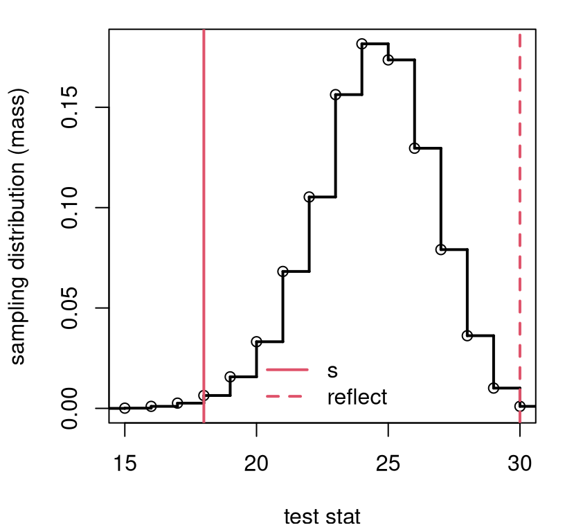
FIGURE 1.3: Using the monty.bern function on the coin-flipping data with $\theta = 0.8$.

Also notice that the statistic, $s_n$, which is in the same location as the previous experiment – it hasn’t changed! – but the sampling distribution is different, as is the reflection of the statistic into the other tail. Even without inspecting the $p$-value, it’s clear that the test is a “close call”. The statistic and its reflection are near the tails, but not way out in the tails. We can make that precise with a $p$-value, but that might not help much in making a final decision. That value is below, along with a comparison from the R library.

c(monty=out$p, lib=binom.test(s, n, p=0.8)$p.value)

##   monty     lib 
## 0.01110 0.01073

If faithful to the default $\alpha=0.05$, then reject $\mathcal{H}_0$. But I wouldn’t bet too much money on it.

Well, there you have it. Now you know how to perform a hypothesis test: just Monte Carlo sample a statistic from the sampling distribution implied by the null hypothesis, and check if your observed statistic is typical (fail to reject) or rare (reject) under that distribution. That’s a mouthful and hard to remember, so I came up with a silly alternative. Just “Monty the null hippopotamus”. You’ll never forget.

It really is just that easy. There’s some art to choosing good statistics – ones with good power, as they say. Power is an important statistical concept, but one that is largely glossed over in this book. In my opinion, it belongs in a second or third course in statistics, for after you have a handle on the notion of the sampling distribution of a statistic. I think that just by following your nose, you can choose a sensible statistic – one with good power – and concern yourself with fine-tuning later. I’ve put a bit about power analysis in §A.2 in case you’re curious, and for completeness. I shall refer to that from time to time so as not to derail focus from other more pressing themes.

There’s also some art to model choice, depending on what data you have. Coin flips are pretty easy in both regards. More widely, there are simple principles that help. I’ll get to those in §3.1, but first in Chapter 2 I’ll show you one more important class of models and tests with the tools we already have. You’ll get lots of practice, beginning with some homework exercises on coin flips.

1.5 Homework exercises

These exercises help gain experience with Bernoulli/binomial tests. We shall return to some of them later with an expanded toolkit.

Ensure that you are using methods outlined in this chapter. Many students will have experience working with Bernoulli/binomial tests in other contexts, from previous classes, other books, or materials found online. Those will be discussed and evaluated in later chapters and homeworks. Deploying non-Chapter 1 methods here will likely not earn full credit.

It is intended that you do these problems with your own code, or code from this book/chapter. I encourage you to check your work with library functions like binom.test. However, check with your instructor first to see what’s allowed. Unless stated explicitly otherwise, avoid use of libraries in your solutions.

#1: More flips

What would you conclude for the coin-flips experiment if more coins were flipped, but the outcomes had the same proportion? That is, suppose you got …

36 heads out of 60 flips (double-sized),
180 heads out of 300 flips (10$\times$).

#2: Silicone wafers

A semiconductor manufacturer claims that 10% of the silicone wafers they produce are defective. In a random sample of 400 wafers, 50 were found to be defective. What do you think?

#3: PVC or copper piping

A building inspector claims that 70% of all homes in Richmond, VA use newer PVC water piping as opposed to copper or other legacy materials. In a random survey of homes in an older neighborhood, 8 out of 15 had PVC. Is this in line with the building inspector’s claims?

#4: GPS speed vs. speedometer

It has been claimed that smartphone maps using GPS underestimate highway driving speeds compared to in-dash speedometers. An experiment was conducted with a team of professional drivers. The driving team recorded the mapping app, GPS-estimated speed when the car was set to cruise at a speedometer reading of 70 mph. Of the 50 readings, 29 of them were too slow (i.e., $<70$ mph). What do you conclude?

#5: Simulation as a means of calculation

This question has nothing to do with data or statistics, but more generally explores the concept of Monte Carlo for calculating probabilities of certain events.

In a certain process, the probability of producing a defective component is 0.07. Calculate the following probabilities using only virtual coin flips (i.e., by Monte Carlo).

In a sample of 250 randomly chosen components, what is the probability that fewer than 20 of them are defective.
In a sample of 10 randomly chosen components, what is the probability that one or more of them is defective?
In a sample of 12 randomly chosen components, what is the probability that the number of defective ones is odd?
(This one is for brownie points.) To what value must the probability of a defective component be reduced such that only 1% of lots of 250 components contain 20 or more that are defective?

#6: One-liner

It is possible to sample from the sampling distribution (generate Ss) via MC for a binomial test with one line of code in R, and crucially without any for loops. Can you figure out how to do that? Calculating the $p$-value can be done, cleanly, with a second line (e.g., using pval.discrete or by hand for $\theta = 0.5$). Maybe you could code both into one long line if you insist.

Hint: generate N*n flips all at once, arrange them in a $N \times n$ matrix and use rowSums on that matrix.

References

Hammersley, J. M., and D. C. Handscomb. 1964. Monte Carlo Methods. London: Chapman & Hall.

Jones, O., R. Maillardet, and A. Robinson. 2009. Scientific Programming and Simulation Using R. Boca Raton, FL: CRC Press.

Stefan, R. C, and T. O. Cheche. 2016. “Coin Toss Modeling.” arXiv Preprint arXiv:1612.06705.

Torcher, K. D. 1969. Art of Simulation. England: Hodder & Stoughton Ltd.

Technically, I should be using uppercase $S_n$ and $Y_1,\dots,Y_n$ because I am entertaining a hypothetical, with a random variable as opposed to actual data values. But for now, I’m not doing that because I don’t want to involve probabilistic expectations. At least not yet; hold your horses for Chapter 3.↩︎
Actually, logarithm was coined by a Scottish mathematician, and algorithm is named after a Persian one.↩︎
A histogram technically provides a mass, sometimes approximating a density, not a distribution which is the sum or integral of a mass or density.↩︎

Monty the Null Hippopotamus