Chapter 8 Bootstrap and permutation
This chapter serves as a warm-up for the next several to come. I want to take you on a little journey before circling back to linear regression (previous chapter) for the grand finale at the end of the book. Broadly, the topic is nonparametric statistics (non-P). I’ll say more about what that is in a moment. This is an unconventional topic for an introductory stats textbook. Sometimes you get a dabble here and there, but I’m giving you five chapters worth starting here. I didn’t encounter non-P until I was in graduate school. Even then I didn’t fully appreciate what was going on. It wasn’t until I taught a class on non-P at VT in 2016, more 10 years after finishing my PhD, that I developed an appreciation.
Larry Wasserman, an eminent Carnegie Mellon statistician, and my academic grandfather (my PhD advisor’s advisor), famously wrote a book called All of Statistics (Wasserman 2004). It’s 450 pages long and doesn’t have any non-P in it. Don’t worry, he wrote another book called, you guessed it, All of Nonparametric Statistics (Wasserman 2006). Both books are available to download for free at those links. They’re targeted to graduate students, and are highly technical. I’m not saying you should read them, at least not yet. They help me make a fun anecdote. By the way, Larry’s advisor was Rob Tibshirani. Rob is the most cited author of articles in “data science” according to Google Scholar. He has the second-most cited author beat by more than 100,000 citations at the time of writing. That’s my academic great-great grandpa! So proud. (We’ve never met, but I have been to dinner with his (biological) son, Ryan. Aren’t you glad you bought my book?)
But I digress. The glossing over of non-P in undergraduate curricula is a shame because it’s a beautiful subject. That’s only part of the reason it features so prominently here. The main reason is computational. Presentation of non-P methods can be obscured by difficult math and asymptotics which – and this is my opinion – undermine their uptake and use in practice. For researchers working on non-P, the goal was to develop statistical methods that could be better trusted because they involved fewer untestable or unrealistic assumptions.
If you’re ever an expert witness involved in a statistical analysis in a courtroom and you use a paired \(t\)-test, say, be prepared to defend your choice of Gaussian distributions for your two populations. With non-P you’re in the clear on that. (More soon.) In spite of that enhanced robustness to scrutiny, there’s a haze of smoke around non-P because people don’t understand what’s going on behind the scenes. It looks like voodoo, and I want to fix that.
Cheap computation is a game-changer. As with material earlier in the book, short algorithms coded in a modern language add a degree of transparency. You can “see” what’s happening in the code. Calculations can be highly accurate with big enough \(N\). No \(n \rightarrow \infty\) asymptotics. Finally, and especially for me and for this book – and maybe this is the same as my second reason – non-P methods showcase the power of thinking through a statistical analysis from first principles via virtualization.
In this chapter I cover two somewhat more modern non-P methods, the bootstrap (Efron 1979) and permutation tests (Dwass 1957). These are, I think, the easiest to understand and so they make for a good warm-up. The bootstrap is particularly powerful, and is perhaps one of the most important computer-based methods in statistics in the last 100-years. So it’s perfect for Monty. And it’s just so simple, which is what makes it beautiful. Bootstrap resampling and permutation tests are quite generic in their approach to inference, and this is a double-edged sword. In later chapters I’ll cover some classical non-P procedures, ones more tailored to particular testing and inference scenarios, lending statistical power (§A.2).
8.1 Non-P
I’ve always thought that nonparametric statistics is a bit of a misnomer. If you read the definition on that Wikipedia page, it doesn’t mention parameters. How can you say what something is not without addressing what’s not not? How can you explain what it means to be disgruntled without addressing what it means to be gruntled?
The main thing that’s “non” about nonparametric statistics is the lack of probability models for the data-generating mechanism. In other words, there are no distributions assumed for the populations that samples come from. For example, no \(Y_1, \dots, Y_n \stackrel{\mathrm{iid}}{\sim} \mathcal{N}(\mu, \sigma^2)\). Since we’re not using Gaussians in this way, or Bernoulli, Poisson, exponential, or otherwise, then we also don’t need their parameters. I think this is where “nonparametric” comes from, but as you can see it’s buried a bit.
I’m going to say “non-P” going forward. That way you’ll think both about the lack of parameters, and the lack of probability distributions for the populations. Look how there’s three p’s (not) there: parameter, probability, and population. This doesn’t mean there aren’t populations at all, nor does it mean we don’t use probabilities or estimate quantities that could easily be called parameters. However, we don’t use those things all together at once to make assumptions about the data-generating mechanism.
Non-P methods still use probabilistic reasoning, like expectation, independence, identically distributed, or the notion of a distribution. But they just don’t commit to a specific distribution dialed in by a small handful of \(p\) parameters \(\theta\) to describe sampled quantities. When \(p\) is just one or two, as it’s for many common distributions, that’s a heavy burden. All \(n\) observations, which could be in the hundreds, are boiled down to two numbers. This is powerful when it works, but is the real world ever that simple?
Instead non-P does a delicate dance around assumptions. One great way to characterize non-P is that the observational data is the distribution. Either it defines an empirical distribution directly (§A.1), like bootstrap resampling and permutation tests of this chapter, or it is defined through some transformation of the data, often their ranks. I don’t want to get too ahead of myself though. I’ll address ranks in Chapter 9.
In this way, non-P methods are more flexible than parametric ones (or just “P”) because they have \(n\) degrees of freedom (DoF) instead of \(p \ll n\). Since we don’t need to estimate any of \(p\) parameters, we don’t lose any DoF for downstream inference. On the other hand though, estimating parameters simplifies things. Distilling \(n\) quantities down to \(p\) provides neat summaries that are easy to keep track of. Ordinary P methods have many closed-form solutions, whereas many non-P ones don’t or must rely on approximation.
In fact, we’ve already seen something like that: the central limit theorem (CLT) from §4.1. Recall that no distribution for the population was assumed. However, samples must be iid and have common mean and variance. No parameters, no tidy distribution, but yes to probabilistic ideas like iid, expectation, etc. Means and variances are labeled \(\mu\) and \(\sigma^2\) for convenience, but they’re not really parameters in the same sense because no distributional form is assumed. Previously, however, our use of the CLT was always in a P context. After committing to \(Y_i \stackrel{\mathrm{iid}}{\sim} \mathrm{Pois}(\theta)\), say, that nailed down \(\mu = \sigma^2 = \theta\), leading to substantial simplification.
The real problem with the CLT is that it only helps if you want to estimate, and understand the sampling distribution of, a sum or average. Although many statistics can be characterized as sums or averages, some cannot like the median. I’ll say more about medians momentarily. Even when the statistic is essentially a sum, like \(s^2\) estimating variance (3.6), it’s often non-trivial to deduce from that the distribution of more readily interpretable variations, like those based on standard deviation. I say “the real problem” but, in fact, many non-P methods use the CLT as a subroutine in some way, but again hold that thought. It’s time for an example.
Jackknife filet-o-fish
Consider the data values below, which come from a survey of measurements of the length of fish, in inches, caught during a competition hosted in the Chesapeake Bay.
y <- c(9.0, 46.2, 9.0, 13.8, 11.5, 18.3, 15.2, 21.0, 11.2, 30.9, 7.1,
  15.2, 18.1, 25.3, 42.6, 32.8, 11.9, 14.3, 8.3, 11.0, 10.5, 10.7,
  36.4, 11.6, 21.7, 26.5, 25.6, 18.8, 55.7, 24.8, 18.5)
n <- length(y)
n
## [1] 31My father-in-law, who fishes in the Chesapeake and likes to tell me about stuff, says they’re some real “whoppers” in there. Two are nearly 5 feet in length, which is enormous. Most are about a foot in size, and none are smaller than six inches, perhaps due to the equipment being used. We’ll visualize the sample momentarily, but I bet you can tell already that the distribution is highly skewed.
Now consider some estimates from the sample that might be of interest to fish-and-game personnel.
## [1] 18.10 12.06As statisticians, we usually want to know more than mere point estimates. What is the sampling distribution for the median? Can a CI be provided? What is the sampling distribution for the sample standard deviation \(S\)? I’m sure you can think of others, but this is plenty for now. How can we answer those questions without assuming some distributional form?
Quick digression on medians, since this is the first time I’m working with them statistically. The notation used for the median of a sample is \(y^{(n/2)}\), or the \(n/2^\mathrm{nd}\) order statistic. The median is the value that separates the top “half” of values from the bottom, when sorted \(y^{(1)}, y^{(2)}, \dots, y^{(n/2)}, \dots, y^{(n-1)}, y^{(n)}\). The min \(y^{(1)}\) and max \(y^{(n)}\) are other important order statistics.
If you have a vector of \(y\)-values in R, like y, you can find the
\(i^{\mathrm{th}}\) largest by sorting the vector and returning the
\(i^\mathrm{th}\) in order. Note that wouldn’t be the most efficient way,
computationally speaking. For more on that, check out
Quickselect. The median is
technically the \((n+1)/2^\mathrm{nd}\) one if \(n\) is odd, or the average of
the \(n/2\) and \(n/2+1\) sorted values when \(n\) is even.
## [1] 18.1 18.1It’s customary to keep it simple and write \(y^{(n/2)}\) regardless. The random analog of the median is \(Y^{(n/2)}\), or similar for any other order statistic. A strange thing about the median, or any other order statistic, is that it’s one of the values (or an average of two) in a sample, not somehow an aggregate of all of the values like many other statistics.
Alright, back to the task at hand. Check this out. Let \(y_{(-i)}\) denote the data set without \(y_i\). In other words,
\[ y_{(-i)} = \{y_1, \dots, y_n\} \setminus \{y_i\}, \]
so that \(y_{(-i)}\) has \(n-1\) observations. There are \(n\) unique such leave-one-out data sets, for \(i=1, \dots, n\).
Suppose each \(y_{(-i)}\) is used to estimate any quantities of interest, like \(y^{(n/2)}_{(-i)}\) and \(s_{(-i)}\) for median and standard deviation, respectively. There would be \(n\) of each of those. Now treat the whole collection of estimates, over \(i=1,\dots, n\), as a sample from an empirical distribution for any estimators of interest. Each represents a quantity that you would have estimated with a different data set sampled from the population – one with one fewer data point, observed \(n\) different ways.
I know it sounds nuts, but we just boarded the crazy train. You’re in for a helluva ride. This is called the jackknife, actually an apt name. John Tukey coined the term by observing that, like an actual jackknife (a folding, pocket knife), it’s a simple tool that can be used to improvise rough-and-ready solutions on the spot, often more efficiently than requisitioning a purpose-built solution. The jackknife is similar to leave-one-out cross-validation (CV), where the word “fold”, like a folding knife, is used to describe each sub-data set made from holding out elements of the original data. I just mention that in case you’ve come across CV elsewhere. CV is very popular in machine learning, and the jackknife is its mommy.
Here is the jackknife in code for medians and standard deviations.
Ymeds.jk <- Ss.jk <- rep(NA, n)
for(i in 1:n) {
  ## so easy with y[-i], removing the ith element of y
  Ymeds.jk[i] <- median(y[-i])
  Ss.jk[i] <- sd(y[-i])
}
Now consider each estimator in turn. We have \(n = 31\) sample medians, \(y_{(1)}^{(n/2)}, \dots, y_{(n)}^{(n/2)}\). One option is to use those directly, and build a CI from their empirical quantiles. This is usually my go-to, but with only 31 samples, it’s hard to be precise about 2.5% and 97.5%. The closest you can get is 3.2% and 93.5%. Another option is to use the samples to calculate moments (means and variances) first, and then deploy a CLT-like approximation with those moments to deduce Gaussian quantiles. Both are approximations which improve with \(n\). I’ve decided to go the Gaussian approximation route here.
## [1] 15.87 18.94Figure 8.1 offers a visual of these quantities alongside a
scatter of the original sample for perspective. The interval is plotted as
red brackets. Both the original median (ymed, filled red diamond), and the
average of jackknife sampled medians (open red diamond) are shown.
plot(y, rep(0, length(y)), ylim=c(-0.5, 2.25),
  xlab="fish length (in)", ylab="", yaxt="n", bty="n")
points(mean(Ymeds.jk), 0, pch=5, col=2, cex=1.5)
points(ymed, 0, pch=18, col=2, cex=1.5)
text(CI.med.jk, rep(0, 2), c("[", "]"), col=2, cex=1.5, pos=3, offset=0)
legend("topright", c("raw median", "avg median"), col=2, pch=c(18, 5),
  pt.cex=1.5, bty="n")
legend("topleft", "[ ] median fishlen CI", text.col=2, bty="n")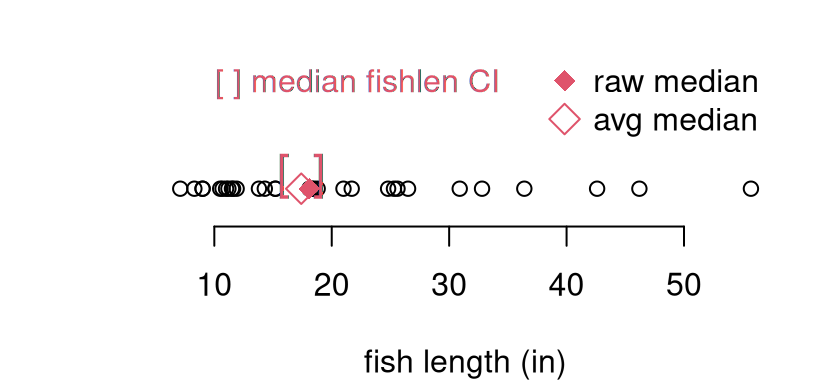
FIGURE 8.1: Jackknife median (open red diamond) and 95% CI (brackets) for the fish length data (open black circles). The raw median on the original data is indicated as a filled red diamond.
We have nothing to compare this to, but the visual is fairly compelling. For my taste, the interval is a bit on the narrow side. This is just based on instinct, and some awareness about jackknife’s limitations. There are operational similarities between the jackknife and MC from earlier chapters. One big difference, however, is that the jackknife is not stochastic. That means it doesn’t involve randomness. Instead of generating synthetic data from a known distribution with fixed parameterization (via the null), the data itself (with one observation removed) is used. Not very many such “simulations” are entertained; only \(n \equiv N\). Consequently, the level of diversity of values, compared to MC, is low.
## Ymeds.jk
## 16.65 16.75  18.2
##    15     1    15
Having three unique values is better than one, which is what you get without a jackknife. I’ll leave it to you to convince yourself that this isn’t just bad luck. If you only remove one point, there can be at most three unique median values in \(y_{(-i)}\) over all \(i\) for any \(n > 4\).
Now for standard deviation; similar options are available, and I’ll stick with a Gaussian approximation.
## [1] 11.29 12.82Again, there’s little (yet) to compare this to. I trust this calculation a bit more since it is based on 30 unique values, as opposed to three in the case of the median.
## [1] 29Ultimately, I’m setting up the jackknife as a straw man. It embodies the spirit of non-P, but has downsides. You don’t get sufficient “good looks” at a diversity of (sub-) samples with just \(n\) examples, or even fewer in the case of the median. A jackknife is a handy tool to have in your pocket, but it’s not a Sawzall.
As I said earlier, many non-P methods, but not all, lean on the CLT – or something like it – in some fashion. Those that don’t involve some pretty fancy mathematics, landing technical details well outside of the scope of this book. Computation with MC is easy by contrast. There will be many instances where I simply quote a mathy result, with a quick pointer to its origin or intuition, and then we get on with drawing a comparison to MC provided in full.
Many applications of non-P involve small data sets – small \(n\). In those settings, it can be hard to characterize how far an asymptotic calculation is from its exact ideal. I much prefer MC in such cases, but you know that already. The jackknife is an extreme example of this. Its performance is tightly coupled to \(n\), and there’s no MC alternative. This makes it somewhat limiting, except as a warm-up.
When the CLT is not involved, one would refer to tables (often published in the backs of textbooks) to obtain percentiles and quantiles for \(p\)-value and confidence interval (CI) calculations in a non-P setting. Producing such tables required hefty computation in their own right. These endeavors comprised statisticians’ early forays into supercomputing. (Think 1960s, vacuum tubes, punch cards, and mainframes occupying entire buildings, and hundreds of hours of compute time and energy.) For some of those, there are now library-based automations, but not for all. I’ll show you a few, but mostly focus on how to do-it-yourself (DIY) with MC and a few handful of lines of R or Python, all in a matter of seconds.
Bootstrap resampling and permutation tests are not only a good warm-up. These are omnibus non-P methods that can be adapted to many contexts. The bootstrap is a direct update to the jackknife, as its creator Efron (1979) explains in the title to that paper: “Bootstrap Methods: Another Look at the Jackknife”. Only \(n\)-many “samples” are not many – not really an empirical sampling distribution. We’re used to getting \(N \geq 10{,}000\) via MC. The bootstrap fixes this.
I think of the bootstrap as a tool for summarizing uncertainty in a way that’s perfect for calculating CIs. Don’t forget you can always invert a CI to set up a test. Permutation tests are more specific, targeting tests of differences in populations, like a non-P alternative to a two-sample \(t\)-test (§5.2). In subsequent chapters, we’ll get even more specific in order to target specialized hypotheses. Enhanced specificity means improved statistical power (§A.2). The more you tailor your assumptions and testing apparatus to the question of interest, the more discerning you can be, statistically speaking.
8.2 Bootstrap
In describing the jackknife above, I’ve all but told you what the bootstrap is. Here it is in one sentence: Instead of deleting each data element, forming \(n\) data sets, sample with replacement and have (almost) as many as you want. It’ll help to be a little more specific. Also, in what follows, I’m going to start from scratch so you needn’t have read about the jackknife, although I shall revisit the fish example to draw a comparison.
Choose a statistic \(s_n = s(y_1, \dots, y_n)\) of interest, like median or standard deviation. In what follows, I’ll drop the \(n\) subscript on \(s_n\) and simply refer to \(s(\cdot)\). I want to use subscripts for something else, and the formalism for arbitary statistics is clumsy anyways. A particular hazard here is estimated standard deviation, which also uses the letter \(s = \sqrt{s^2}\), following Eq. (3.6). I’ll try to make any distinctions clear when necessary, but mostly it should be automatic from context.
Now, instead of calculating the statistic(s) directly on the original data \(y \equiv (y_1, \dots, y_n)\), resample those data values \(Y^\star = \mathrm{resample}(y)\) with replacement and then calculate the statistic(s) on that, virtual data \(S = s(Y^\star)\). Another way to write that is
\[ Y^{\star} \stackrel{\mathrm{iid}}{\sim} \mathrm{Unif}\{y_1, \dots, y_n\} \quad \rightarrow \quad S = s(Y^\star). \]
This is even easier in code. Here is an example of what I mean with the median statistic.
Ystar <- sample(y, n, replace=TRUE)    ## always take n = length(y) samples
Ymed <- median(Ystar)                  ## this is s(Ystar)
c(Ymed, ymed)
## [1] 15.2 18.1Notice how the calculation turned out different than when using the original data directly. Why is that? Because resampled \(Y^\star\) is different from the original data vector \(y\). In particular, \(Y^\star\) has some entries missing,
## [1] 18.3 21.0 18.1 32.8 11.9 11.0 11.6 26.5 18.8 24.8 18.5leading to 18 unique values, rather than \(n = 31\). Since the sampled version \(Y^\star\) still has \(n\) entries, then it must have some of the original data values represented more than once.
##
##  7.1  8.3    9 10.5 10.7 11.2 11.5 13.8 14.3 15.2 21.7 25.3 25.6 30.9
##    1    1    2    3    1    2    3    1    1    2    2    3    1    3
## 36.4 42.6 46.2 55.7
##    1    1    2    1
See that some are even in triplicate. It’ll be yet again different when you
try it on your own machine as sample is random. In
drawing this so-called bootstrap sample \(Y^\star\), we implicitly treat the
original data \(y_1, \dots, y_n\) as if it were the entire population. Doing
that over and over again is not unlike MC from earlier chapters. Rather than
using an assumed distribution under a null hypothesis, we now treat the
observed data as the distribution. It’s a finite, discrete distribution with
\(n\), not necessarily unique, values.
The “with replacement” caveat is crucial. Resampling \(n\) items from \(n\) items
without replacement is the same as randomly permuting them, without
otherwise altering its composition. This changes nothing in practical terms
if we’re working under an iid assumption, where order doesn’t matter.
Technically, we’re making an
exchangeability
assumption which is weaker than iid, but that distinction isn’t really
important here. (I just say these things so my nerdy colleagues don’t
complain.) Take-home message: don’t forget replace=TRUE.
Figure 8.2 lays it all out in a diagram. I contemplated using an algorithm environment, but ultimately thought a schematic would look more slick. The total number of bootstrap samples is \(B\). This is like \(N\) for MCs in earlier chapters. I could have used \(N\) here, too, but I didn’t for a few reasons. One is that you see \(B\) a lot in the literature. Besides always being quick to jump on bandwagons, I think it’s helpful to make a distinction between ordinary MC, and a bootstrap MC. Recall that all MC means is that you’re using random sampling in your calculation. Using \(B\) reminds you it’s sampling observed data with replacement, instead of generating from a distributional family under \(\mathcal{H}_0\).
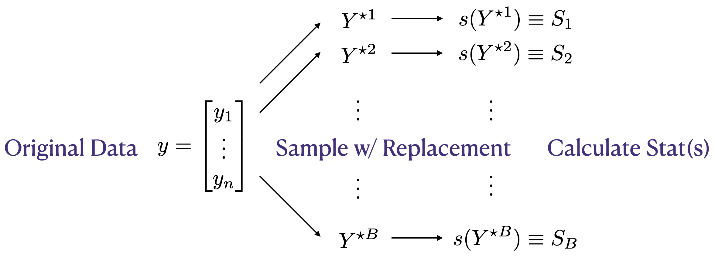
FIGURE 8.2: Bootstrap resampling diagram, yielding samples \(S_1, \dots, S_B\) comprising an empirical distribution for \(s(Y) \equiv s(Y_1, \dots, Y_n)\).
Finally, \(B\) can’t be as big as you want, like \(N\) can. The largest reasonable \(B\) is linked to \(n\). Consider the simple but silly case of \(n=2\). It’s easy to count that there are only three unique possible \(Y^\star\)s up to permutation: \((y_1,y_1), (y_2,y_2), (y_1,y_2)\). It doesn’t make a whole lot of sense to ask for \(B=10{,}000\) in that case. But three bootstrap samples is already more than the jackknife which would only have two, each being of size just one. Obviously \(n=2\) is an extreme example. I’ve left counting the number of unique bootstrap samples, in greater generality, to you as an exercise in §8.5. Spoiler alert: it’s really big even for smallish \(n\).
It’s worth remarking that Figure 8.2 applies to the jackknife
as well. Just take \(B = n\) and don’t sample with replacement, but take
\(Y^{i\star} = y_{(-i)}\). Since a jackknife implementation is just a for
loop, so is the bootstrap. Easy code, but the result is surprisingly rich, at
least compared to a jackknife. The something-for-nearly-nothing aspect is
what led Brad Efron to call it
the bootstrap.
Efron, like Tukey, worked at the interface between statistics and machine learning, so he was better at naming things than most classical statisticians. “Bootstrap” combines two uses of the term from elsewhere. One, in the vernacular but also common in the business world, refers to the impossibility of “pulling yourself up by your bootstraps”. The other is common in technical usage, like in computer engineering, where a self-sustaining process is started with very little external input. A bootloader, short for bootstrap loader, is a program that starts up, or “boots” your computer. In the case of bootstrap resampling, and indeed of the jackknife, that “very little external input” is \(y_1,\dots, y_n\). Nothing else except an iid assumption, and not even that in all cases, is required. At some point it helps to choose a statistic, \(s(\cdot)\), but even that can be delayed ’till later. Let me show you.
Fish length via bootstrap
Here’s the bootstrapping loop. Notice how I’m saving each sample, and not calculating a statistic. This is the “Sample w/ Replacement” step in Figure 8.2.
B <- 10000
Ystar <- matrix(NA, nrow=B, ncol=n)
for(b in 1:B) {
  Ystar[b,] <- sample(y, n, replace=TRUE)
}
Those samples may be used to calculate a distribution for whatever statistic I want. This is the “Calculate Stat(s)” step in the figure. Let’s begin with the median.
Since the median is one of \(n= 31\) values from the original data, it’s worth checking how many unique ones, and with what frequency, ended up in the bootstrap collection.
## Ymeds
## 10.7   11 11.2 11.5 11.6 11.9 13.8 14.3 15.2 18.1 18.3 18.5 18.8   21
##    1    2   18   37  109  302  531  786 2453 1468 1341 1154  816  516
## 21.7 24.8 25.3 25.6 26.5
##  304  109   39   12    2
This is many more than the paltry three that we got with a jackknife. This distribution is depicted in Figure 8.3. Still, these 19 values are not \(B= 10^{4}\) values. Using quantiles directly for CI calculation could be fraught with inaccuracy. So again I opt for a Gaussian approximation.
That interval is overlayed as purple brackets on the histogram in Figure
8.3. To reiterate, that histogram is not the original
sample, but rather bootstrap sample of medians, Ymeds. However, the range
of the \(x\)-axis is the same as in Figure 8.1 in order to keep
perspective. Compared to the jackknife, the bootstrap interval is much wider,
owing to a greater diversity of samples. Just on instinctual grounds, I like
this new interval a lot better.
hist(Ymeds, xlim=range(y), main="", xlab="fish median length")
points(mean(Ymeds), 0, pch=5, col="purple", cex=1.5)
points(ymed, 0, pch=18, col=2, cex=1.5)
text(CI.med.jk, rep(0, 2), c("[", "]"), col=2, cex=2, pos=3, offset=0)
text(CI.med, rep(0, 2), c("[", "]"), col="purple", cex=2, pos=3, offset=0)
legend("topright", c("raw median", "boot avg median"),
  col=c("red", "purple"), pch=c(18, 5), pt.cex=1.5, bty="n")
legend("right", "[ ] new boot CI", text.col="purple", bty="n")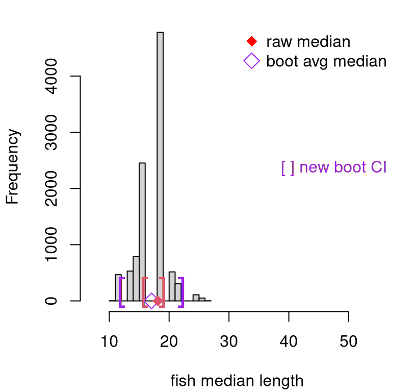
FIGURE 8.3: Bootstrap sampling distribution of medians (purple), compared to jackknife (red).
Original median \(y^{(n/2)}\) is plotted as a red diamond. This is the same as in Figure 8.1, along with those red jackknife brackets. The purple circle, however, is calculated as an aggregate of bootstrap samples. Bootstrap aggregating is sometimes referred to as bagging and, again owing to the diversity of samples from the empirical distribution of the original data, lends a degree of robustness to any point estimate.
I’d like to spend a brief moment on testing. Suppose some pundit asserted that the median catch size for competitive anglers fishing in the Chesapeake was 20 inches. We would not be able to reject that hippopotamus with these data because 20 is well within the 95% interval. And if someone quibbled that they don’t trust our modeling assumptions, we can chirp back that our analysis was non-P. All we assumed is that the data are iid.
Now we move on to standard deviation. This is easy with bootstrap resamples already in hand. Storing all of those samples could be memory-intensive if \(B\) and \(n\) are both big, but that pays off in compute time (and in code) if you have more than one statistic in mind.
Since estimated standard deviation, \(s\), is derived from a squared average of all observations in the data – or in this case in a bootstrap resample – we obtain many more unique values.
## [1] 9992Observe that this is close to, but less than, \(B = 10^{4}\), the total number of samples. It must have been the case, on
## [1] 8occasions, that one bootstrap resample \(Y^{\star i}\) was identical to another \(Y^{\star j}\) up to permutation. That can happen. It’s even possible to get \(Y^{\star i} \equiv y\), up to a reshuffling, in which case \(S_i = s(y_1, \dots, y_n)\). A homework exercise explores this further.
Since there are so many unique values, there’s little harm in calculating a CI via quantiles, as opposed to using the CLT.
See Figure 8.4, which additionally shows the full bootstrap sampling distribution of estimated standard deviation \(S\). Again, this new bootstrap interval is much wider than the jackknife analog.
hist(Ss, main="", xlab="fish length sd")
points(mean(Ss), 0, col="purple", pch=5, cex=1.5)
points(s, 0, pch=18, col="purple", cex=1.5)
text(CI.s.jk, rep(0, 2), c("[", "]"), col=2, cex=2, pos=3, offset=0)
text(CI.s, rep(0, 2), c("[", "]"), col="purple", cex=2, pos=3, offset=0)
legend("topleft", c("raw median", "boot avg sd"),
  col=c("red", "purple"), pch=c(18, 5), pt.cex=1.5, bty="n")
legend("topright", "[ ] new boot CI", text.col="purple", bty="n")
FIGURE 8.4: Bootstrap sampling distribution of standard deviations (purple), compared to jackknife (red).
I encourage you to contrast those quantile-based intervals with a CLT version. I’d guess they’d be quite similar.
Return on investment
Recall the return on investment (ROI) example from §2.5.
Consider ROI for individual companies who use the particular IT product first.
So as not to write over y and n – I want to re-use those later – I’ll use
yc and yi. Industry values, comprising yi will come later.
Recall from the histogram of these quantities in Figure 2.3 that the distribution appears heavy-tailed. Consequently, an analysis based on Gaussians in the homework exercise of §2.6, if you did that one, and later in §5.4, is potentially flawed.
Suppose there is interest in performing an analysis based on the sampling distribution of averages. I’ve coded that up below. This time I’m not saving each individual bootstrap resample, just the sample average statistic. You get to decide what you want to do as a software developer (or book author).
Ycbars <- rep(NA, B)
for(b in 1:B) {
  Ycbars[b] <- mean(sample(yc, length(yc), replace=TRUE))
}
CI.c <- quantile(Ycbars, c(0.025, 0.975))
CI.c
## 2.5% 97.5%
## 7.071 18.104Figure 8.5 provides a visual of this CI, with a histogram summarizing the original data overlayed. According to this view, individual company ROI is positive. We would reject the hypothesis that ROI is zero, because zero falls well outside the CI.
hist(yc, main="", xlab="ROI")
text(CI.c, rep(0, 2), c("[", "]"), col=2, cex=2, pos=3, offset=0)
legend("left", "mean ROI CI", text.col=2, bty="n")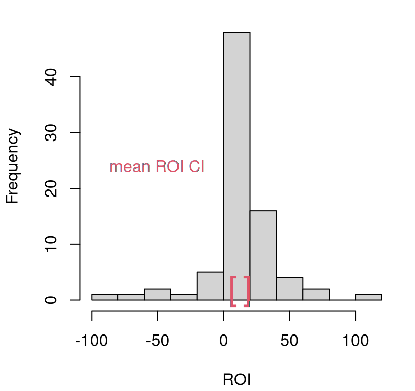
FIGURE 8.5: Company average ROI CI via bootstrap resampling, with original data histogram overlayed for reference.
In the homework question of §2.6 you were asked to test if \(\mu = 15\), representing the industry average. We would not be able to reject that either. But that’s not the right way to conduct a two-sample analysis. There’s uncertainty in both estimates. One option is another bootstrap.
yi <- roi$industry
Yibars <- rep(NA, B)
for(b in 1:B) {
  Yibars[b] <- mean(sample(yi, length(yi), replace=TRUE))
}
Next, form the distribution of their difference, just like in a two-sample \(t\)-test from §5.2, but without assuming Gaussianity.
Ybds <- Yibars - Ycbars                      ## bd is short for "bar diff"
CI.diff <- quantile(Ybds, c(0.025, 0.975))
CI.diff
## 2.5% 97.5%
## -3.536 8.260Zero is in that interval, so we wouldn’t be able to reject that the two samples have the same mean. Evidence is mounting that the “professional” analysis behind the negative ad campaign was suspect. From every which angle you look, it seems like companies that use that IT product have the same mean ROI as does the industry at large.
You might have noticed, in both examples above, that I avoided explicit \(p\)-value labeling and nomenclature. You certainly can be probabilistically precise about the visual assessments in the figure above. For example, here’s the probability that that average ROI is bigger than zero.
## [1] 0That’s pretty strong evidence. You could multiply that by 2 to make it “two-sided”; same thing with the two-sample version based on differences.
## [1] 0.4356But neither is strictly a \(p\)-value, by definition, because we didn’t sample under a null hypothesis. Rather, we used that CI as the inverse of a hypothesis test. Some may quibble with this. I’m fine with it, but as you can tell, I’m a bit cavalier about these things – about most things, except hard work and no excuses. Those are important. You could argue that, implicitly, our \(\mathcal{H}_0\) was that the two populations were independent. But again, this is the opposite of the typical setup. A classical null would specify that the two hypotheses are the same, and seek to reject that in favor of evidence otherwise.
One might conclude that bootstraps are limited in this sense, if all tests
must invert CIs. Perhaps. That’s not a completely accurate portrayal, but it
would take us into a rabbit hole to correct. I’d rather focus on how its
most basic form is flexible in other, possibly even more useful ways. You can
do so much with simple for loop and sample, basically without
modification, in so many settings. For example, you can bootstrap ordinary
least squares (OLS) from §7.4, and conduct inference for
linear models without placing a Gaussian assumption on responses. Just
treat each training data pair as a single unit, \(z_i = (x_i, y_i)\), bootstrap
resample over \(z_1, \dots, z_n\), save estimates of slope and intercept and
make histograms. You can do it with predictions too. I’ve left these to you
to explore in your homework.
Strangely enough, there’s also something called the parametric Bootstrap, and other ways to use similar resampling ideas toward other ends. This comes in handy when you’re ok with P, but you find resampling more convenient than the pure, null hypothesis MC. There are good reasons to proceed in this fashion, but I’ll leave it to you to track those down. Some pointers are provided in §8.4.
8.3 Permutation
A permutation test specifically targets two-sample testing. Whereas a bootstrap can be appropriated to test two samples, it can be somewhat underpowered (§A.2), as nothing about it is targeted to that application specifically. It’s just two independent bootstraps stitched together. Whereas it’s hard (but not impossible) to place a bootstrap analysis within a conventional hypothesis testing framework, this is rather more natural for the permutation test.
It goes like this. Suppose \(Y_1, \dots, Y_{n_y} \stackrel{\mathrm{iid}}{\sim} F_Y\) for some generic, unspecified distribution \(F_Y\), and \(X_1, \dots, X_{n_x} \stackrel{\mathrm{iid}}{\sim} F_X\) similarly.
\[\begin{align} \mathcal{H}_0 &: F_Y = F_X && \mbox{null hypothesis (“what if")} \tag{8.1} \\ \mathcal{H}_1 &: F_Y \ne F_X && \mbox{alternative hypothesis} \notag \end{align}\]
In some sense this setup is ridiculous, since it’s overly generic. Every sample is a little different than another one for some reason or another. The real question is: what differences can be detected with limited data? As with any statistical test, that hinges on your choice of statistic, and how you study its sampling distribution. That’s your wedge.
With permutation tests, it’s common to develop a statistic that can be applied to the combined sample
\[\begin{equation} s(y, x) = s(y_1, \dots, y_{n_y}, x_1, \dots, x_{n_x}), \tag{8.2} \end{equation}\]
but, ultimately makes contrasts between \(y\) and \(x\) vectors, of length \(n_y\) and \(n_x\) respectively, through simpler statistics applied separately to the two groups of data. For example,
\[\begin{equation} s(y, x) = \bar{y} - \bar{x}, \quad \mathrm{sd}(y) - \mathrm{sd}(x) \quad \mbox{ or } \quad \mathrm{sd}(y) / \mathrm{sd}(x). \tag{8.3} \end{equation}\]
It may look as if I’ve created some overly cumbersome notation for a simple thing. It wouldn’t be the first time. The important thing about Eq. (8.2) is that although the first \(n_y\) are labeled as \(y_i\) and the latter \(n_x\) as \(x_i\), when we actually use \(s(\cdot, \cdot)\) the \(x\)’s and \(y\)’s will be jumbled up. You’ll see. In that case, say for \(s(y, x) = \bar{y} - \bar{x}\), what happens is that the first \(n_y\) values, no matter what they are, shall be averaged and likewise the last \(n_x\). Then their difference is returned.
Why jumble things up? Because the null hypothesis (8.1) says that the distributions of \(Y\) and \(X\) are the same (\(F_Y = F_X\)). So if we were to shuffle the full deck of data before feeding into \(s(\cdot, \cdot)\), e.g., obtaining \(s(x_{12}, x_{7}, y_{3}, x_{8}, y_{9}, y_{2}, \dots)\), in effect treating some \(y\)’s as \(x\)’s and vice-versa when calculating \(s(y,x)\), that shouldn’t change anything on average, because \(X\) and \(Y\) have the same distribution. Or do they? That’s what the permutation test helps us determine.
Let \(n = n_y + n_x\) be the size of the combined sample. Consider all \(n!\) shufflings, or permutations, of the combined data and calculate \(s(\cdot, \cdot)\) for each one, providing \(s_1, \dots, s_{n!}\). This is your sampling distribution for the statistics, which is a bit of a misnomer since the procedure (iterating over all permutations) is deterministic. While the statistics will indeed distribute themselves, meaning they will be spread out and you can compare that spread to the observed/unpermuted one, the distribution is not stochastic.
This is all, of course, nonsense since you can’t iterate over \(n!\) anything for \(n\) of any reasonable size. When \(n=60\), combining two size thirty samples, say, you get \(n! > 10^{81}\) which is near in number to what many scientists estimate to be the total count of all atoms in the universe. Good luck enumerating all of those, and storing a statistic for each!
Instead, most applications of permutation tests sample at random from available permutations, which is the same as saying sample without replacement from the combined \(n\)-sized collection. Choose a number of permutations \(P\) as large as computation or practical limitations allow (like \(N\) or \(B\)), and calculate \(S_1, \dots, S_P\). These are random, and have a probabilistic distribution, as long as each permutation is sampled at random.
In other words, it’s like the bootstrap as diagrammed in Figure
8.2, but (a) with two samples pasted together; (b) use
replace=FALSE; and (c) use a statistic \(s(\cdot)\) that targets contrasts
between the two groups (8.3). It’s bizarre that the opening line
to the Wikipedia page reads “A permutation test … is an exact statistical
hypothesis test.”9 It’s
not in most applications. You can’t believe everything you read on the
internet. Also like with bootstrap resampling, some of the sampled statistics
may be identical to others if they involve the same first \(n_y\) and last \(n_x\)
values.
More fish
Suppose that the fish-length survey was repeated on another day, and lengths were recorded below.
x <- c(23.4, 18.1, 37.8, 32.5, 26.1, 22.0, 15.0, 32.2, 37.5, 19.2, 15.9,
  31.4, 13.0, 14.8, 24.1, 21.6, 34.6, 28.0, 27.1, 25.2, 26.1, 37.6,
  33.1, 14.7, 25.0)
Let’s first test by averages, which may be calculated as follows. I find it helpful to combine the two samples, straight away in order to calculate the test statistic. That way I can test things out before using a similar calculation later in the random permutation loop.
nx <- length(x)
ny <- length(y)     ## formerly n, but now n is for combined sample
yx <- c(y, x)
n <- length(yx)                                   ## same as nx + ny
bdiff <- mean(yx[1:ny]) - mean(yx[(ny + 1):n])    ## this is s(.)
c(bdiff, mean(y) - mean(x))
## [1] -5.005 -5.005I chose the variable name bdiff, short for “bar difference”, or difference
in \(\bar{y}\) and \(\bar{x}\). Writing the statistic somewhat generically for
the combined sample, and checking that it works as desired, is helpful for the
next step.
P <- 10000
Bds <- rep(NA, P)
for(p in 1:P) {
  YXs <- sample(yx, n)                               ## rand permutation
  Bds[p] <- mean(YXs[1:ny]) - mean(YXs[(ny + 1):n])  ## s(YXs)
}
Figure 8.6 shows the distribution of sampled statistics along with the observed one, and it’s reflection, overlayed. This is a nice looking histogram, and one that seems to favor \(\mathcal{H}_0\). A \(p\)-value calculation adds precision.
## [1] 0.0822hist(Bds, main="", xlab="differences in means", xlim=c(-11, 13))
abline(v=bdiff, col=2, lwd=2)
abline(v=-bdiff, col=2, lty=2, lwd=2)
legend("topright", c("obs", "reflect"), lty=1:2, lwd=2, col=2, bty="n")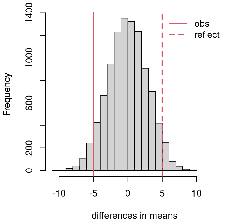
FIGURE 8.6: Permutation distribution for differences in mean fish length.
Although the \(P = 10^{4}\) samples is but a small fraction of \(n! > 10^{75}\), I’m reasonably confident that the calculation is accurate. Indeed, a substantial proportion (around 79%) of those sampled permutations led to identical statistics, because they amounted to reshuffled \(y\)’s to the first \(n_y\) locations and \(x\)’s to the last \(n_x\). Any doubts can be put at ease with larger \(P\).
## [1] 0.7873So we weren’t able to reject that the distributions were the same by targeting differences in averages. How about differences in estimated standard deviation? You could try either of the options in Eq. (8.3). One advantage to going with a difference, as opposed to a ratio, stems from familiarity with two-tailed testing. Ratios of positive statistics are always positive; recall that we preferred one-tailed tests of two sample variances in §6.2.
As with the bootstrap, you could potentially save the random permutations and re-use them with another statistic. The fancy word for that is caching. Alas, I didn’t think ahead. Cut-and-paste it is …
sdiff <- sd(yx[1:ny]) - sd(yx[(ny + 1):n])
Sds <- rep(NA, P)
for(p in 1:P) {
  YXs <- sample(yx, n)
  Sds[p] <- sd(YXs[1:ny]) - sd(YXs[(ny + 1):n])
}
Figure 8.7 shows the sampling distribution of differences in estimated standard deviation obtained from sampled permutations. This is a closer call than many recent examples. The \(p\)-value says …
## [1] 0.0336… reject \(\mathcal{H}_0\) at the 5% level, and determine that the samples likely came from a different distribution (\(F_Y \ne F_X\)) because they differ in their standard deviation.
hist(Sds, main="", xlab="differences in stdevs", xlim=c(-7,10))
abline(v=sdiff, col=2, lwd=2)
abline(v=-sdiff, col=2, lty=2, lwd=2)
legend("topright", c("obs", "reflect"), lty=1:2, lwd=2, col=2, bty="n")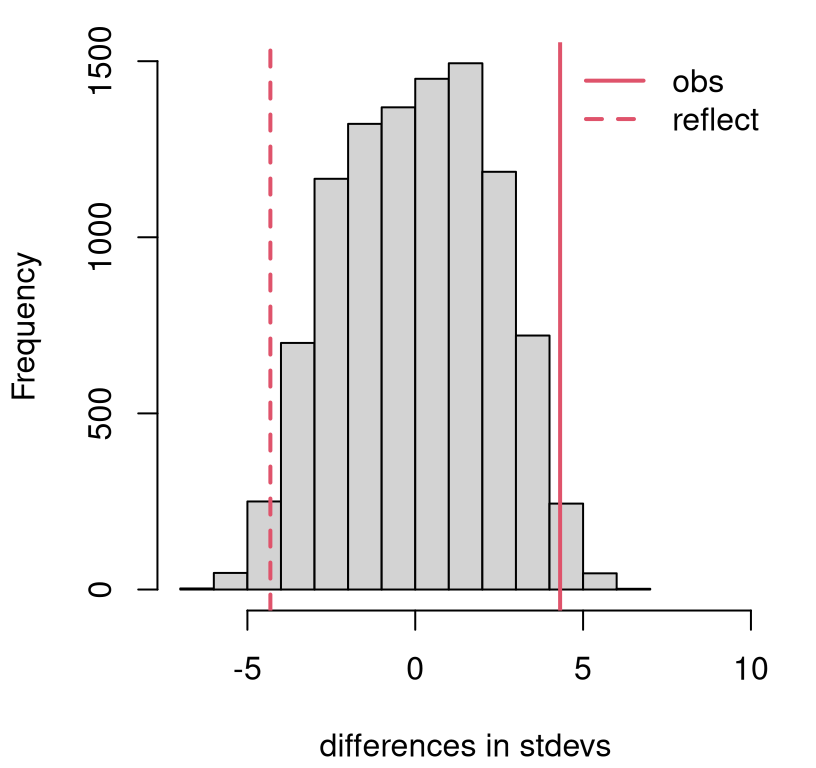
FIGURE 8.7: Permutation distribution for differences in standard deviation of fish lengths.
A word of caution though: if you keep testing the same hypotheses, over and over again with different statistics, you’re bound to be snagged by a multiple testing hazard. Recall our discussion in §6.4. Twenty borderline tests at the 5% level yield one false positive on average. We ran the test (only) twice targeting very different aspects, so I’m not that concerned about it. But if you keep hunting around for something, you’ll probably find it. In that sense, every null hypothesis is doomed.
More ROI
Now consider a similar pair of tests for ROI. First, set up the combined sample and calculate observed test statistics.
yx <- c(roi$company, roi$industry)
ny <- length(roi$company)
nx <- length(roi$industry)
n <- ny + nx
bdiff <- mean(yx[1:ny]) - mean(yx[(ny + 1):n])
sdiff <- sd(yx[1:ny]) - sd(yx[(ny + 1):n])
This time, I shall combine average- and \(s\)-sampling into a single
for loop.
Bds <- Sds <- rep(NA, P)
for(p in 1:P) {
  YXs <- sample(yx, n)
  Sds[p] <- sd(YXs[1:ny]) - sd(YXs[(ny + 1):n])
  Bds[p] <- mean(YXs[1:ny]) - mean(YXs[(ny + 1):n])
}
I’ll skip the histogram visuals and jump straight to \(p\)-values. Be sure to get those inequalities the right way around. Don’t be “that guy” who reports a \(p\)-value bigger than one.
##    avg     sd
## 0.6256 0.0000
Careful here: zero doesn’t really mean zero. It means \(\psi < 1/P = 10^{-4}\),
which is pretty small. This result is consistent with earlier analysis.
Figure 2.3 clearly indicates distributions with different
variances, and this makes sense considering that numbers in roi$industry are
aggregates. So they clearly come from different distributions \(F_Y \ne F_X\).
Those differences are not in location, but rather in scale.
8.4 Wrapping up
I normally mention software along with the method in order to make a direct
comparison, but here I’m doing it at the end of the chapter. One reason is
that, at least for bootstrap (and jackknife) and permutation tests, I’m not a
big fan of the library options. It’s not that the libraries aren’t good, but
rather the nature of the beast means that they offer lower value compared to
DIY MC. These methods are just simple for loops with re-sampling alongside
simple statistical summaries. That’s pretty easy. By the time you read all the
documentation for the library, you could have DIY’d.
Take boot (Canty and Ripley 2024) built into R, for example. The main function, also called
boot, is clearly intended for more ambitious applications than the
introductory ones I presented in this chapter. It seems straightforward
enough to provide boot(data, statistic, replicates), for example as boot(y, mean, B) using our setup for ROI from §8.2. But that
doesn’t work because the second, statistic argument must itself take two
arguments. The contents of those arguments depend on other boot
specifications, etc., determining exactly how resampling is to be deployed.
There are many good reasons to do things a little differently than I’ve
described in this chapter, but that’s for another course. There are whole books
on this stuff (Davison and Hinkley 1997).
I eventually figured out that I needed the following if using the default of
stype="i", which utilizes indices in the observed data for resampling.
The reason for this is complicated, but ultimately sensible. No doubt
the authors landed on this setup after much deliberation. Rather than
resampling data values directly, the boot function samples indices from
1 to \(n\), like I <- sample(1:n, n, replace=TRUE), and then applies those
indices to the data, like y[I]. This is a little more flexible, allowing
your data to be a matrix or data.frame where you may wish to bootstrap over
rows. That can be handy if you’re bootstrapping OLS, like in the homework
exercises. The data object can even be more complex, like a list. But for
our simple setup, this extra scaffolding represents an additional layer of
complexity.
library(boot)
bout <- boot(roi$company, avgstat, B)
CI.boot <- rbind(byhand=CI.c,
  lib=quantile(bout$t, c(0.025, 0.975)))
CI.boot
## 2.5% 97.5%
## byhand 7.071 18.10
## lib 7.059 18.16That’s pretty much the same result, but possibly more work. One really nice
thing about boot is that it automates parallelization, over multiple cores
on your machine. That can be important with really big \(B\) and/or with a
statistic that’s computationally demanding to compute. There are some other
nice features which come in handy as you entertain other forms of bootstrap,
like weight-based, parametric, residual bootstrap, and so on. I won’t go over
those. Davison and Hinkley (1997) is an excellent reference, and you can find others
in the boot documentation (?boot). The package also provides an
implementation of the jackknife.
Permutation tests are provided by the perm library (Fay and Shaw 2010), but it’s
somewhat limited in options. As far as I can tell, only a test based
on differences in averages is provided, at least as pertains to our
modeling setup.
library(perm)
pval.perm <- permTS(roi$company, roi$industry)$p.value
pvals <- c(pvals[1], lib.avg=pval.perm)
pvals
## avg lib.avg
## 0.6256 0.6210That’s basically the same result. It wouldn’t be hard to write your own
monty.perm library that worked more like boot, allowing for specification
of an arbitrary statistic as an argument to the function in order to automate
aspects of permutation tests. Speaking of good homework problems …
8.5 Homework exercises
These exercises help gain experience with bootstrap and permutation-based procedures. Although some questions are mathematical in nature, when it comes to application, the procedures are purely numerical. Some problems refer to questions performed via parametric procedures in earlier chapters. These are just a selection. Pretty much any of the earlier questions could be entertained with non-P. Likewise, many questions targeting non-P procedures could be entertained with P instead, so long as you choose an appropriate distribution for modeling.
Do these problems with your own code, or code from this book. Unless stated explicitly otherwise, avoid use of libraries in your solutions.
#1: Counting resamples
Let your training data comprise of \(n\) unique values, \(y_1, \dots, y_n\). That means no duplicates. Answer the following questions about resampling which are relevant for the bootstrap in an iid modeling situation.
- How many distinct resamples of size \(n\) are possible? Since we are in an iid modeling context, two samples are not distinct if one is a permutation of the other.
- What is the probability that a random resample matches a permutation of the original data?
- Among the distinct bootstrap samples from #a, what is the probability of observing one with at least one repeated value?
#2: Library function monty.boot
Write a function called monty.boot that automates bootstrap tests and
intervals with an arbitrary statistic. Take inspiration from boot, as
described in §8.4 above, but yours will be much simpler.
The function prototype should look like monty.boot(y, stat, B, s0=NULL)
with sensible defaults like stat=mean, assuming y is a vector, and
B=10000. A user should additionally be invited to provide some other function
for stat that could be calculated for y. Return a CI for the
statistic and calculate an a \(p\)-value, via inversion, if the user optionally
provides a s0 to compare to.
As a bonus, embed your new monty.boot within monty.t from
§3.5 and monty.var from §6.5,
providing the option of a non-P one-sample CI and test for means and
variances, respectively. In this application it’s fine to hard-code
stat=mean or stat=var as appropriate. Don’t just cut-and-paste code.
Call your new function.
Hint: many of the following questions are easier after this one is squared away.
#3: Filling potato sacks
A sack of Idaho potatoes typically weighs 110 lbs. A new potato-sack filling machine was purchased and tested on twelve bags. Their weights, in lbs, are provided below.
Use bootstrap resampling to answer the following.
- Does the average fill weight agree with the nominal specification of 110 lbs?
- Provide a 95% CI for the average fill weight.
#4: Revisit heights
Revisit the heights data from Chapter 2, whose analysis was based on a Gaussian distribution. In the exercises of §2.6, you were asked to entertain a Gamma distribution. Now use the bootstrap in order perform a non-P test. Are women in my class of average height? Additionally provide a CI for their heights.
#5: Revisit TV lifespans
Question #2 from §3.5 involved data on times-to-failure of a certain new smart TV. Use a bootstrap to provide a CI for the lower quartile of failure times, in years. Lower quartile is sometimes notated as \(y^{(n/4)}\). It separates the bottom 25% from the top 75%, in the same way that the median separates the bottom half from the top half.
#6: Revisit re-insurer claims
Question #3 from §3.5 involved data on insurance claims. You were asked to use a quirky distribution I called the scale-1 Pareto. Repeat parts #c and #d from that exercise with non-P via the bootstrap.
#7: Revisit rent OLS inference
Question #15 from §7.8 considered data on rent as predicted by size. You may find the data in rent.csv, linked from the book webpage.
Revisit parts #a–#c via bootstrapped OLS. In particular, provide sampling distributions for the proportion of variability explained by the fit, and any regression coefficients that allow you to say if square-feet is a useful predictor. Finally, provide a CI for the additional cost per 1,000 square feet.
I suggest going back to the formulas for \(b_0\) and \(b_1\), but you could opt
to use coef(lm(...)). Note, however, you do not need to use any of the
standard errors, etc., that lm objects provide. The idea of this question
is that you’re not making a Gaussian assumption, because a bootstrap is
non-P. If you’re assuming a Gaussian, you can’t use any of the results that
are based on it. Finally, it will help to use the sample function to
generate indices so that you can resample \((x_i, y_i)\) pairs together, as a
single unit. Optionally, you could figure out how to use boot to automate
things, but actually I think this is harder.
#8: Revisit rent OLS prediction
This question carries on from #7 above, completing question #15d from §7.8 via a non-P bootstrap. Use your bootstrap samples to overlay error bars derived from a CI on prediction.
Hint: each bootstrap sample gives you a line, and so the collection of all \(B\) lines can be used to form that CI, tracing out error bars in the scatterplot. Taking the additional uncertainty into account via a PI is harder, because that involves an additional distribution assumption. I’m not suggesting you do that here.
#9: Library function monty.perm
Write a function called monty.perm that automates permutation tests with an
arbitrary statistic. The function prototype should look like monty.perm(y, x, stat, P). Use sensible defaults like stat=mean with y and x
vectors, and P=10000. Your user should additionally be able to provide
some other, possibly custom-built, function for stat that could be
calculated for y and x. Automate the formation of the combined yx,
and its randomly permuted YXs, saving the stat as differences over P
iterations. Return an appropriate \(p\)-value.
As a bonus, embed monty.perm within monty.t (§5.4)
and monty.var (§6.5), providing the option of a non-P
two-sample test. In this application it’s fine to hard-code stat=mean or
stat=var as appropriate. Don’t just cut-and-paste code. Call your new
function.
Hint: many of the following questions are easier after this one is squared away.
#10: Cloud seeding
Simpson, Olsen, and Eden (1975) report on an experiment that was conducted to determine if seeding clouds with silver iodine increases rainfall. Fifty-two clouds were seeded in this way, and fifty-two other (but otherwise similar) clouds were not seeded as controls, and the amount of rain in acre-feet was saved. These data may be found on DASL, or as clouds.csv on the book webpage.
- Treat the rows of the data as paired and conduct a non-P test via the bootstrap to determine if there is a difference in average (i.) or median (ii.) rainfall for seeded and unseeded (control) clouds.
- Now treat the rows as unpaired and conduct a permutation test with the same statistics in part #a.
What do you conclude?
#11: Revisit heights again
Revisit the two-sample heights experiment from §5.2 which combined women’s heights from my class (Chapter 2) and new ones from the VT women’s basketball team. Perform a non-P permutation test to determine if these women’s heights come from the same distribution.
#12: Memory-enhancing supplements
Solomon et al. (2002) report on a study where elderly adults were randomly assigned to take Gingko, via an over-the-counter supplement, and others to take a placebo. After four weeks the subjects had their memory evaluated by several objective neuropsychological tests and subjective ratings, which were summarized into a single score. Those scores are provided in memory.RData linked from the book webpage and may additionally be found on DASL.
Use a permutation test, with any statistics you decide, in order to determine if Ginkgo supplements have any effect on memory.
References
boot: Bootstrap R (s-Plus) Functions.
Maybe that’ll change before this book goes to print.↩︎