Chapter 9 Non-P location
This chapter is the non-P version of Chapters 2 and 5, combining one-sample and two-sample (unpaired and paired) location tests, respectively. But I’m going to do them in reverse, because in this presentation the one-sample version is a special case of the two-sample one.
All three tests derive from a paper by Wilcoxon (1945), although there are some other players involved as I’ll explain. Frank Wilcoxon was a chemist by training and trade, who discovered statistics through a study of Fisher’s papers in the course of his own research for the chemical companies that he worked for. Wilcoxon’s main insight, statistically, stemmed from a study of the distribution of ranks, which is what now underpins much non-P analysis.
Converting raw data into ranks represents clever insight, in my opinion, and really opened things up for me as I was learning about non-P. There are some beautiful mathematics in there, but we’ll only scratch the surface on that. As usual, MC with ranks is super simple, in part because ranks are permutations of positive integers – something we already know lots about from the previous chapter.
Sometimes, the procedures presented in this chapter are referred to as Wilcoxon \(t\)-tests. I don’t like that. Although Wilcoxon’s procedures target the same setting as parametric \(t\)-tests, for one and two samples (and paired), there’s no \(t\) statistic, nor \(t_\nu\) distribution. Sometimes statistical texts generically use the letter \(t\) for “test statistic”. I think that’s confusing.
I want to acknowledge a book by Conover (1999), which is where I first
learned the material here, and in the next few chapters, while teaching a
non-P class at Virginia Tech (VT). That book was a great resource, but also
one that feels antique when set in a contemporary (computing) landscape. The
tables of quantiles and percentiles in the back of the book are now obsolete
given q* and p* functions in R. In fact, it was a desire to modernize
that material that led, eventually, to the idea of my Monty. First, I figured
out how to avoid the tables (the “math” way), and then I figured out how to do
the MC, which I now prefer.
While writing these passages, and on scale-based tests in Chapter
11, I stumbled across an R package called ANSM5 (Spencer 2024). That
package supports a book (Smeeton, Spencer, and Sprent 2025) which, in turn, was also a new discovery
for me. The spirit of that book, and its accompanying software, is quite
similar to my Monty. They even do MC. I’ll admit that at first that bummed
me out. Their book is more broad on non-P. Mine focuses a bit more on
statistical foundations.
I realized in particular that much of the software in that package could be
used as a benchmark, especially for routines that are not available in base R.
I have not done that here, because I already had library-based alternatives in
place. ANSM5 will come in handy later in Chapter 11. I wanted to
give them a shout now because they deserve it, and in case the reference is
helpful to you.
9.1 Ranks
Many classical non-P procedures involve ranks. Ranks are intimately related to order statistics, which were first introduced as a digression in §8.1. In a way, ranks are the inverse of an order statistic. The rank of a member \(y_i \in \{y_1, \dots, y_n\}\) is its index \((i)\) in sorted order \(y^{(1)}, \dots, y^{(n)}\).
Ranks are easier to describe with a formula if there are no duplicated values in \(\{y_1, \dots, y_n\}\), i.e., no ties in the ranks. Let’s consider that case first. The rank \(r_{n,i}\) of \(y_i\) is
\[\begin{equation} r_{n,i} = \sum_{j=1}^n 1_{\{y_j \leq y_i\}} \quad \mbox{for unique} \quad \{y_1,\dots,y_n\} \tag{9.1} \end{equation}\]
where \(1_{\{\cdot\}}\) returns 1 when the expression in \(\{\cdot\}\) is true and 0 otherwise. So the rank of a data point is the count of the number of other data points it is greater than, plus itself. Subscript \(n\) in \(r_{n,i}\) is intended to indicate a relationship to the other \(y_1,\dots,y_n\) values. Often I simplify to \(r_i \equiv r_{i,n}\) when that connection is explicit from context.
If you found that description cumbersome, here are some examples in R to help. Suppose we had some data values, like those below. I just made them up. Again, no ties for now.
What is the rank of \(y_4 = 9\)? The formula says …
## [1] 3Or, by inspection, we can see that 9 is the third largest because 6 and 3 are the only ones that are smaller.
Eq. (9.1) would be a cumbersome way to calculate all \(n\) ranks. A
better algorithm might go something like this. First sort the data, but rather
than return the sorted values just return the sorted order. This is what the
order function does in R. (These aren’t the ranks, yet. Just the first
step.)
## [1] 6 3 4 11 7 2 10 9 8 1 5In other words, to sort y, take index 6 first, then 3, and so
on. Checking …
## [1] 3 6 9 11 12 14 23 36 37 73 85Increasing – perfect. According to o, take index 4 in position 3. And so that’s the rank \(r_4 = 3\) of \(y_4\). Said
another way, a rank tallies when a particular data value would be taken in
sorted order. So a rank is the order of the order.
##    [,1] [,2] [,3] [,4] [,5] [,6] [,7] [,8] [,9] [,10] [,11]
## oo   10    6    2    3   11    1    5    9    8     7     4
## r    10    6    2    3   11    1    5    9    8     7     4
If you’d like, you can check any of those via Eq. (9.1) above. Now
we have all the ranks for all \(n\) elements. See what I mean by ranks being
the inverse of an order statistic? Note that an order statistic isn’t the
same as the order function, though they’re related. R’s rank
automates order of the order. That’s what we’ll use going forward,
but this wasn’t waste because now you know how it works!
The main reason to use rank(y) rather than order(order(y)) is how the
former automates handling ties. The rank function has several options for
this, and we’re going to use the default which is ties.method="average".
It goes like this: take the order of the order, as above. Call these the
OO-ranks. Any ties will receive consecutive ranks by the OO-method. That’s
not good, because it would arbitrarily favor otherwise equivalent measurements
with lower or higher ranks, depending on the number of ties. So, replace the
OO-ranks of those points (the ones with ties) with their average OO-rank.
Here’s a new \(y\) vector to experiment with, augmenting the other one with a few ties.
First find OO-ranks.
Then, for the duplicated ones, replace with an average.
dups <- unique(y[duplicated(y)])
r <- oor
for(d in dups) {
  inds <- which(y == d)
  r[inds] <- mean(r[inds])
}
I’m not sure this implementation is the most efficient, but it’s fairly transparent. Fortunately, the library provides a nice automation, and we can check that the two agree.
##     [,1] [,2] [,3] [,4] [,5] [,6] [,7] [,8] [,9] [,10] [,11] [,12]
## r     13  8.5    2    3   14    1    6   12   11    10     4   8.5
## lib   13  8.5    2    3   14    1    6   12   11    10     4   8.5
##     [,13] [,14]
## r       6     6
## lib     6     6
Rank \(r_2\) has a \(1/2\) fractional part because \(y_2\) is duplicated, causing two consecutive ranks to be averaged. Rank \(r_7\) is not fractional, but rather shares the rank 6 as the average of three consecutive whole numbers: 5, 6, 7.
Why are ranks helpful? One practical thing is that they make the sample unitless. Whether \(y\) is measured in miles-per-gallon, or kilometers-per-liter, ranks \(r\) of \(y\) go from \(1, \dots, n\). Ranks preserve the order of data values, while homogenizing the gaps between them. You can have a heavy tail in one or both directions, or multiple modes causing data values to clump and spread and clump and spread again, etc. Rank them and they’ll be evenly spaced. There’s always a gap of one between one rank and the next, modulo ties.
Finally, and perhaps most importantly for statistics, ranks impose an implicit empirical distribution (§A.1) after dividing by \(n\). I encourage you to read more about that in the Appendix. What it means for us here is that the uniform distribution, \(\mathrm{Unif}(0,1]\), is sensible for modeling \(r/n\). Fixating just on the \(n\) particular rank values, a discrete uniform will do. So when working with ranks in a non-P context, you boil an unknown distribution down to the very simplest one: uniform. What a trip!
If you don’t completely follow, which would be understandable because I just distilled a highly technical argument occupying whole chapters of other textbooks down into a paragraph, don’t worry. I just wanted to give you some context. We’re not going to need a handle on all of that to get busy with testing. Just appreciate that ranks offer a transformation of observed data values, from whatever values they had originally down to integers between 1 and \(n\), inclusive.
9.2 Wilcoxon/Mann–Whitney
The Wilcoxon rank sum test is a test for differences in means for samples from two populations. It’s sometimes also known as the Mann–Whitney test, as it was developed independently around the same time (Mann and Whitney 1947). The setup is the same as for permutation tests. Suppose \(Y_1, \dots, Y_{n_y} \stackrel{\mathrm{iid}}{\sim} F_Y\), and \(X_1, \dots, X_{n_x} \stackrel{\mathrm{iid}}{\sim} F_X\) similarly. Implicitly, the test is about determining if \(F_Y = F_X\) or not, but unlike the permutation test which is somewhat generic through a choice of testing statistic, a Wilcoxon test specifically targets means.
\[\begin{align} \mathcal{H}_0 &: \mathbb{E}\{Y\} = \mathbb{E}\{X\} && \mbox{null hypothesis (“what if")} \tag{9.2} \\ \mathcal{H}_1 &: \mathbb{E}\{Y\} \ne \mathbb{E}\{X\} && \mbox{alternative hypothesis} \notag \end{align}\]
There are variations targeting other aspects, such as variance, but those are coming later in Chapter 11. Also like the permutation test, the Wilcoxon test works on the combined sample of size \(n = n_y + n_x\). Let \(r_i^{(y)}\) and \(r_j^{(x)}\) denote the rank assigned to \(y_i\) and \(x_j\) in the combined sample, respectively, for all \(i=1,\dots, n_y\) and \(j=1, \dots, n_x\). If there are ties, then assign an average rank as described in §9.1. Although it helps to keep track of them separately, as \(r_i^{(y)}\) and \(r_j^{(x)}\), don’t forget that ranks are assigned on the combined sample.
It’ll help to introduce a running example to make everything concrete. Data values below come from a survey of Washington Metro riders at various stations in Virginia (\(y\)) and Washington DC \((x)\) during a particular commute hour. These numbers tally how many riders said that they used a prepaid paper fare card. These were introduced when Metro opened and which are now being phased out in favor of the newer plastic, credit-card-like SmarTrip cards.
First, form the combined sample and then rank.
The portion of those ranks corresponding to \(y\) and \(x\), \(r{(y)}\) and \(r{(x)}\), respectively, may be extracted as follows.
Several statistics get used with Wilcoxon rank sum tests, depending on context and software, but all of them are based around the sum of the ranks assigned to the first, \(y\), group.
\[\begin{equation} \bar{r} \equiv \bar{r}^{(y)} = \sum_{i=1}^{n_y} r_i^{(y)} \tag{9.3} \end{equation}\]
Actually, it’s equivalent to use the sum of the second, \(x\), group, which is why I drop the \((y)\) superscript. It doesn’t matter which you pick. Just keep track of what you’re doing and be consistent. The test comes out the same, either way. (I encourage you to verify.)
## [1] 72Note that I’m using a bar over \(r\), as \(\bar{r}\), which is a notation usually reserved for an average rather than a sum. We could take the average instead, i.e., divide by \(n_y\). For the MC method I take you through momentarily, it doesn’t matter. For the math way, we’d have to multiply \(\bar{r}\) by \(n_y\) before using it if we prefer to use an average. I’ve chosen not to do that because this is known as the Wilcoxon “rank sum” test, not the “rank average” test, and I don’t want to be too confusing. I’ll admit that my choice of \(\bar{r}\) as the label for the statistic is unconventional. Many simply write \(t = \sum_{i=1}^{n_y} r_i^{(y)}\), and I’ve already explained why I don’t want to use the letter \(t\).
People always find this statistic (9.3) curious. You have two
samples, but the test only uses the ranks of one of them, say \(r^{(y)}\). I
saved rx above, but actually I don’t need it for anything. When you think
about it, though, the \(x\) sample is “felt” through ry, because those values
were calculated from the combined sample. Ranks \(r^{(x)}\) are there
implicitly, in the in-between spaces of the ranks of \(r^{(y)}\). So the
distribution of \(R^{(x)}\) is felt through \(R^{(y)}\).
In a moment I’ll take you through the MC, and then through the math. In both cases, the idea is as follows. If \(F_Y = F_X\), under the null10, then ranks of \(Y\) will look like ranks of \(X\) in the combined sample, \(R^{(y)}\) and \(R^{(x)}\). You won’t be able to tell the difference, because they came from the same population. Therefore, any summary of those ranks, like their sum or average, will also look the same, on average. Once we understand the sampling distribution of \(\bar{R}\), we may compare that to \(\bar{r}\) from observed data.
One last note is relevant for both ways. Under the null hypothesis
\[\begin{equation} \mathbb{E}\{\bar{R}\} = \frac{n_y(n_y + n_x + 1)}{2} = \frac{n_y(n+1)}{2}. \tag{9.4} \end{equation}\]
This is pretty easy to show. The sum of all \(n\) ranks, assuming they’re distinct (i.e., no ties) is \(\sum_{i=1}^n i = n(n+1)/2\). I suspect you’ve seen sums of finite series before, but if not that’s fine. The particular one in question here is known as a triangular number. Instead of summing up all \(n\) ranks, \(\bar{R}\) sums just \(n_y\) of them. It doesn’t matter which ones when it’s uniformly at random. By similar logic, the caveat “no ties” isn’t really needed since ties are replaced with average ranks.
Wilcoxon test by MC
Sampling ranks is as easy as randomly permuting \(\{1,\dots,n\}\).
N <- 1000000
Rbars <- rep(NA, N)
for(i in 1:N) {
  Ryxs <- sample(1:n, n)
  Rys <- Ryxs[1:ny]
  Rbars[i] <- sum(Rys)
}
According to Eq. (9.4), the mean of this distribution may be calculated as follows.
## [1] 100 100You can see that the theoretical value and MC calculation agree. \(\mathbb{E}\{\bar{R}\}\) is important here in order to reflect the observed statistic over the mean for our favorite visual. Use either the theoretical value, or its MC estimate, and the visuals come out about the same. Graphics aren’t rocket science, but that’s not the main reason for showing you. I’m building trust for later when we really need Eq. (9.4) for the math way. In the meantime, Figure 9.1 provides a histogram summary of MC samples of \(\bar{R}\) with observed and reflected statistics overlayed.
hist(Rbars, main="")
abline(v=c(rbar, 2*Rmean - rbar), col=2, lty=1:2, lwd=2)
legend("topright", c("obs", "reflect"), lty=1:2, lwd=2, col=2, bty="n")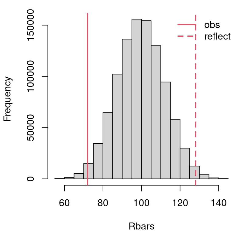
FIGURE 9.1: Sampling distribution of \(\bar{R}\) with observed \(\bar{r}\) for the Metro fare card data, and its reflection overlayed.
This is a close call. Looks like a reject to me, but let’s be sure with a \(p\)-value calculation.
## [1] 0.02222Indeed.
Ok, now I want to pivot slightly and talk about ties in the combined sample
resulting in averaged ranks. Here is a new data set to work with. These
values come from a follow-on study with an otherwise similar setup: counting
paper fare card rides on Metro during a particular commute hour at stops in DC
and Maryland (MD). So as not to overwrite the earlier VA (y) and DC (x)
values – I want to use them later – this time I’ll work with MD as y2 for
\(y\) and DC as x2 for \(x\).
y2 <- c(67, 94, 83, 98, 35, 73, 29, 36, 60, 105, 34, 84, 89, 76, 79, 92,
  49, 97, 46, 32, 104, 60, 61, 59, 98, 101)
x2 <- c(107, 114, 87, 102, 85, 94, 109, 91, 99, 59, 97, 92, 103, 90, 43,
  108, 61, 111, 87, 112, 109, 115, 89, 105, 109, 83, 35, 114)
It’s easy to see some duplicated entries. A pair of 87s jumps out at me. There are many more than that, and I’ll be more precise later. What I want to do first is carry out the analysis as if this whole ties thing was no big deal. Perhaps it is no big deal. Tracing steps from above, with suitable changes in symbols, …
yx2 <- c(y2, x2)
ryx2 <- rank(yx2)
ny2 <- length(y2)
ry2 <- ryx2[1:ny2]
nx2 <- length(x2)
n2 <- ny2 + nx2
Next calculate \(\bar{r}\) and run the MC loop for \(\bar{R}\). This time I’m allowing some variables from the earlier VA/DC analysis to be overwritten because I don’t need them later.
Rbars <- rep(NA, N)
for(i in 1:N) {
  Ryxs <- sample(1:n2, n2)
  Rys <- Ryxs[1:ny2]
  Rbars[i] <- sum(Rys)
}
I’ll skip the histogram visual and jump right to the \(p\)-value.
## [1] 0.000422Ok, so easy reject. However, this virtualization was not faithful to the
observational data. We know that there are ties in the ranks of the
observed values, but there are no ties (by construction) in any of the virtual
ranks sampled within the MC loop. Each is a random permutation \(1, \dots, n
\equiv\) n2 without any averaged values. What to do?
There’s actually no playbook for this, at least when it comes to MC. I’m not the first person to use MC for statistical testing. But as far as I’m aware, I’m on the vanguard of its application to the Wilcoxon rank sum test, and therefore so are you. I’m sorta making it up as I go. So feel free to expand or modify things and see what happens. People have thought about it some when it comes to the math way I’ll present next, but I’m hoping you’re going to find that unsatisfying. What I’m about to show you is better, or at least more flexible.
The idea here, as with any MC, is to tailor a virtualization to what you know about the data-generating mechanism. Mimic what little you know, or additionally wish to assume, based on what you observe. The goal is to explore variability of the (rank sum) statistic within the confines of the null hypothesis (9.2) and the nature of observational data. So begin with assessing the situation. How far off are things from the rough-and-ready no-ties solution above?
Let’s count ties. I used duplicated in §9.1 on raw data
values. This time, I think table will give a more compact summary, and I’ve
done it on the ranks themselves. There are many good options long as you’re
careful.
##
##  2  3
## 13  1
Thirteen ranks are duplicated, and one appears in triplicate. What to do
about that? How about randomly generating a similar number of ties through
averaging, before randomly permuting those ranks? This is a little tricky to
implement because it only makes sense to average consecutive ranks. The code
file rank_ties.R, available on
the book webpage, contains a rank.ties function that randomly inserts
rank-averages. For more on this, see §B.2. Here’s a
little demo of how we shall use it for the current analysis.
First, generate 13 degree-2 ties in raw ranks ranging from 1 to the combined
sample size n2 \(\equiv n_y + n_x = n\).
## $ranks
##  [1]  1.0  2.0  3.5  3.5  5.5  5.5  7.0  8.5  8.5 10.0 11.0 12.0 13.5
## [14] 13.5 15.5 15.5 17.0 18.5 18.5 20.0 21.5 21.5 23.0 24.0 25.0 26.0
## [27] 27.0 28.0 29.0 30.5 30.5 32.0 33.0 34.0 35.0 36.0 37.5 37.5 39.0
## [40] 40.5 40.5 42.0 43.5 43.5 45.0 46.0 47.5 47.5 49.0 50.0 51.5 51.5
## [53] 53.0 54.0
##
## $uniq
##  [1]  1  2  7 10 11 12 17 20 23 24 25 26 27 28 29 32 33 34 35 36 39 42
## [23] 45 46 49 50 53 54
A quick scan of consecutive ranks reveals fractional values that come from averaging. The choice of which pairs for averaging is random, so if you run this on your own machine, you’ll likely get a different outcome.
The rank.ties function is designed to be daisy-chained. So you can
take ranks from one call and pass them into another as follows. The
key ingredient is keeping track of any remaining unique, non-average
ranks in rd2$uniq.
rd3 <- rank.ties(rd2$ranks, 1, 3, rd2$uniq)    ## with 1 degree-3 tie
tab <- table(rd3$ranks)
table(tab[tab > 1])
##
## 2 3
## 13 1Now we have 13 averages from duplicates and 1 from a triplicate. A note of caution, though, when daisy-chaining: do the bigger ties first. That is, first do degree 3, and then degree 2. The larger the degree, the harder it is to find runs of that length. If some ranks are eliminated as runs of degree three because they’re already averaged in a run of degree two, you could end up in a spot where the code can’t find the ties you’re looking for. I didn’t do that above, but I will below.
So first, randomly generate ties, then randomly permute them. Otherwise, the
setup is the same as earlier, where we ignored ties. It must be said that
this new MC is much less efficient, computationally speaking, than the earlier
one. My rank.ties implementation uses a while loop (so we have nested
loops here) in order to iterate over tie possibilities. This incurs
substantial overhead. It’s possible that could mitigated with a more clever
implementation. To assess the damage, I’ve added some timing code.
tic <- proc.time()[3]                             ## stopwatch start
Rbars <- rep(NA, N)
ranks <- 1:n2                                     ## ranks without ties
for(i in 1:N) {
  rd3 <- rank.ties(ranks, 1, 3)                   ## one degree-3 tie
  rd2 <- rank.ties(rd3$ranks, 13, 2, rd3$uniq)    ## plus 13 degree-2 ties
  Ryxs <- sample(rd2$ranks, n2)                   ## randomize over ranks
  Rys <- Ryxs[1:ny2]                              ## rest as usual
  Rbars[i] <- sum(Rys)
}
toc <- proc.time()[3]                             ## stopwatch stop
First, a \(p\)-value calculation.
##   ignore      ack
## 0.000422 0.000472
That’s not much different than we had before. It could be that having more ties, as a proportion of the total ranks, would lead to a more dramatic effect. I draw comfort from exploring both options, and having a variation that uses stochasticity (i.e., random ranks) in a way that’s faithful to my observational data.
Having the number of ties in each MC sample mimic patterns in the data makes sense. The way I did it above is only one of potentially many possibilities. You could, for example, posit that the maximal tying degree has a Poisson distribution, and similarly the number of ties at each degree could be Poisson. I’ll leave that to you as an exercise in §9.5. Again, that’s just one idea.
Considering the extra computational effort,
## elapsed
##   6.515
which is substantial, one wonders if such small differences are worth the hassle. What’s nice about this is that it’s relatively easy to entertain, in terms of human effort. You don’t have to be a clever mathematician. One only needs to come up with a way to virtualize, and randomize over, a feature observed in data. Any way you wish to do that is legitimate, so long as you explain/justify relative to other reasonable alternatives.
Wilcoxon test by math
If \(Y_i\) and \(X_j\) are iid from the same distribution (9.2), and there are no ties, then their ranks on the combined sample should resemble a random permutation of integers \(\{1,\dots,n\}\), for \(n= n_y + n_x\). The \(n_y\) ranks assigned to the first group, should look like a random selection of those integers. Therefore, the distribution of the rank sum statistic (9.3), \(\bar{R}\), may be obtained by considering the distribution of the sum of \(n_y\) integers, selected without replacement from \(\{1, \dots, n\}\).
The number of ways of forming a sum of \(n_y\) integers from \(n\) is \({ n \choose n_y}\). If each way is equally likely, then \(\mathbb{P}(\bar{R} = k)\), for some positive integer \(k \leq \sum_{i=1}^n i = n(n+1)/2\), may be found by counting the number of different subsets of size \(n_y\), from integers \(\{1,\dots, n\}\), that add up to \(k\), and dividing by \({ n \choose n_y}\).
\[ \mathbb{P}(\bar{R} = k) = \frac{\mathrm{SSP}(k, n_y, \{1,\dots,n\})}{{ n \choose n_y}} \]
Subset sum problems (SSPs) are, in general for any set (we’re using \(\{1,\dots,n\}\)), NP-hard. NP-hard means that there’s no known polynomial-time algorithm in \(n\) for all \(n_y\) and \(k\). That’s not quite right. What it actually means is that if you could solve the SSP in polynomial time, then you would also be able to solve a bunch of other intractable problems fast, because those problems belong to an equivalence class (of NP-hard problems). That is a subtle distinction.
Quick digression on SSPs, which I find fascinating. There are lots of seemingly “toy” problems out there like SSP that involve counting how many ways you can do this or that, or other. They seem like games without any real applications, but eventually one comes around. It sure is handy when a solution is ready off-the-shelf. There’s a connection between SSP and a Hollywood movie called The Man Who Knew Infinity, based on a book by Robert Kanigel. Both are a biography of Indian mathematician Srinivasa Ramanujan who was interested in counting things.
I won’t spoil it; but if you like the genre, it’s up there along with: The Imitation Game, about the famous/first computer scientist Alan Turing and code-breaking during World War II; The Theory of Everything about Stephen Hawking and the origins of the universe; and A Beautiful Mind about John Nash and game theory.
Alright, back to SSP and computing. There are some clever approximations
and solvers for special cases. In
ranks.R, available on the book
webpage, I provide mass and distribution functions, called dranks
(implementing \(\mathbb{P}(\bar{R} = k)\)) and pranks (for
\(\sum_{\ell=1}^k \mathbb{P}(\bar{R} = \ell)\)), respectively, which use a
SSP solver library in R. Check this out …
source("ranks.R")  ## note: these are not vectorized
c(d=dranks(rbar, ny, nx), p=pranks(rbar, ny, nx))    ## using k or l = rbar
## d p
## 0.002403 0.011009Here, I’m following the convention in R that density (or mass) functions start
as d* and distribution functions as p*, like dnorm and pnorm. For
more details on these functions and their implementation, see
§B.3. Figure 9.2 provides the mass function
for \(\bar{R}\) corresponding to \(n_y = 10\) and \(n_x = 9\) from the first
Metro VA/DC example. Overlayed are the observed and reflected
\(\bar{r}\)-values calculated earlier.
rgrid <- 50:150
dr <- rep(NA, length(rgrid))
for(k in 1:length(rgrid)) dr[k] <- dranks(rgrid[k], ny, nx)
sfun <- stepfun(rgrid[-1], dr)
plot(sfun, xlim=c(50, 165), xlab="rbar",
  ylab="mass dranks(rbar, ny, nx)", main="", lwd=2)
abline(v=c(rbar, 2*Rmean - rbar), col=2, lty=1:2, lwd=2)
legend("topright", c("rbar", "reflect"), lty=1:2, col=2, lwd=2, bty="n")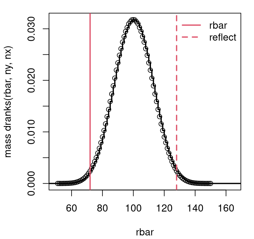
FIGURE 9.2: Exact rank sum sampling distribution for Metro VA/DC example without ties.
This view is quite similar to Figure 9.1. The observed statistic is in the left tail, so a \(p\)-value may be calculated as follows.
##      mc   exact
## 0.02222 0.02202
It looks like our MC is highly accurate. If observed \(\bar{r}\) were in the right
tail, we would usually provide lower.tail=FALSE to a p* function. But
this is not implemented by pranks. I was being lazy. Imagine we had
observed the reflected value of the statistic instead, which is in the right
tail. In that case, provide …
## [1] 0.02202In other words, take away the integral from left.
In R, there’s a distribution function called pwilcox (and similarly
dwilcox, qwilcox and rwilcox), but it works with a shifted statistic:
\[ \bar{r}' = \bar{r} - \frac{n_y(n_y+1)}{2} \quad \mbox{ so that } \quad \mathbb{E}\{\bar{R}'\} = \frac{n_y n_x}{2}. \]
I’m not sure what the reason for this shift is, but I did warn you that several similar statistics were used with Wilcoxon tests.
## [1] 0.02202So pwilcox does the same thing as my by-hand pranks function. It has
the advantage of offering a lower.tail=FALSE option, but rather less
transparency in the underlying calculation.
The name of this function, which uses “wilcox” rather than “wilcoxon”, was a
source of confusion to me for some time. I would say “Wilcox test” (wrong)
rather than “Wilcoxon test” (right). Just be careful. The dude’s name is
Wilcoxon, not Wilcox. Adding another layer to confusion, there’s a
wilcox.test library function automating things. But it does not perform a
“Wilcox test”, because that’s not a thing. It does a Wilcoxon test.
##      mc   exact    lilb
## 0.02222 0.02202 0.02202
Now that was for the case where there were no ties. All of that discussion about randomly permuting ranks and solving SSPs relies on having ranks filling \(\{1,\dots, n\}\). Ties lead to fractional, duplicated and skipped ranks. There’s no simple way to count things in this context, because those ties, etc., can be anywhere. MC, as \(N \rightarrow \infty\) offers the only exact way to work with the sampling distribution in this case. We saw that things didn’t change much, and the same is true here.
Consider my second MD/DC Metro fare card example which had 13 duplicates
and one triplicate. What if we just use pranks, pwilcox or the library
function directly, ignoring the ties?
pval2.mc.ties <- 2*mean(Rbars <= rbar2)    ## Rbars still for to MD/DC
pval2.exact <- 2*pranks(rbar2, ny2, nx2)
pval2.pwil <- 2*pwilcox(rbar2 - ny2*(ny2 + 1)/2, ny2, nx2)
c(mc=pval2.mc, mc.ties=pval2.mc.ties, exact=pval2.exact, pwil=pval2.pwil)
## mc mc.ties exact pwil
## 0.0004220 0.0004720 0.0004403 0.0004403These new “exact” calculations are in agreement with one another, and in close agreement with previously calculated MC \(p\)-values. Yet the library function gives a different number along with a warning.
## Warning in wilcox.test.default(y2, x2): cannot compute exact p-value
## with ties
##
## Wilcoxon rank sum test with continuity correction
##
## data: y2 and x2
## W = 166, p-value = 6e-04
## alternative hypothesis: true location shift is not equal to 0A \(p\)-value of \(\psi = 6 \times 10 ^{-4}\) is pretty close to those other estimates, but the warning together with the message about “continuity correction” suggests something new is afoot. What’s happening?
This is the central limit theorem (CLT; §4.1) in action. Subtracting off the mean (9.4) is the easy part, but dividing by the standard error of \(\bar{R}\) is rather more involved. I’m just going to quote the result here so we can see what the software is doing.
\[ Z = \frac{\bar{R} - \frac{n_y(n+1)}{2} }{ \sqrt{\frac{n_y n_x}{n(n-1)} \sum_{i=1}^n r_i^2 - \frac{n_y n_x(n+1)^2}{4(n-1)}}} \sim \mathcal{N}(0, 1) \quad \mbox{ as } n \rightarrow \infty \]
That standard error is intense! Someone worked hard. It’s not at all clear that, for fixed \(n\), this is any better than using the exact result in the presence of ties. Both represent an approximation in this case.
r2sum <- sum(ryx2^2)
np1 <- n2 + 1
nm1 <- n2 - 1
z.numer <- rbar2 - ny2*np1/2
v <- (ny2*nx2/(n2*nm1))*r2sum - ny2*nx2*np1^2/(4*nm1)
z <- z.numer/sqrt(v)
pval2.clt <- 2*pnorm(-abs(z))
pval2.clt
## [1] 0.0006258This matches what the library provides with exact=FALSE (meaning use CLT)
and correct=FALSE (meaning don’t make a continuity correction).
c(clt=pval2.clt,
  lib.cF=wilcox.test(y2, x2, exact=FALSE, correct=FALSE)$p.val,
  lib.cT=wilcox.test(y2, x2, exact=FALSE)$p.val)
## clt lib.cF lib.cT
## 0.0006258 0.0006258 0.0006460You get a slightly different result with the default of correct=TRUE.
Continuity correction is common when approximating a distribution for discrete
quantities with a continuous one (i.e., Gaussian). It leads to a slightly
more accurate result, which in this case isn’t much different.
## [1] 0.000646I’m just showing you for full transparency. It’s pretty in the weeds,
splitting hairs, and much ado about nothing when it comes to a \(p\)-value that
leads with three zeros. If I’m being honest, I wasn’t exactly sure about the
continuity correction until I downloaded the source code for
R, and searched the archive for
“wilcox.test”.11 This is the beauty of an open-source project, like R.
No smoke and mirrors. Back to Wilcoxon tests … When it comes to which
statistic, and how to approximate with ties, I’m pretty open to good
judgment.
On a pen-and-paper exam, a CLT version is doable especially if the exam provides \(\sum_{i=1}^n r_i^2\). You can’t exactly do a MC, or solve SSPs problems, without a computer. I think this is the main reason why textbooks provide this approximation, historically speaking, not because it’s actually better than something else. In a modern context, the CLT can still come in handy when \(n\) is large. This is when it’s approximation is most accurate, and solving SSPs can be computationally fraught. Remember, SSPs are NP-hard, which means things get bad as \(n\) gets big.
Any of the four or five methods, depending on how you count them, are probably fine if the \(p\)-value is far from 0.05. Perhaps worry more about it when you have lots more ties, as a proportion of the total, and your \(p\)-values differ substantially from one method to the next (near 0.05). In that situation, I’d caution against rejecting the null.
9.3 Signed ranks
If the Wilcoxon rank sum test is the non-P analog of a two-sample \(t\)-test, then the Wilcoxon signed ranks test is the non-P paired version.12 Hypotheses (9.2) and data-generating mechanism are the same (\(F_Y\) and \(F_X\), respectively), but we presume that the data come as \((x_1, y_1), \dots, (x_{n'}, y_{n'})\), where each pair \((x_i, y_i)\) is observed under similar circumstances, or are otherwise linked. Notice I’m using \(n'\) not \(n\) to count the total number of pairs. The reason for that will be apparent soon.
Just like with a paired \(t\)-test, define \(d_i = y_i - x_i\), or vice-versa for \(i=1,\dots,n'\). The signed ranks test makes an additional assumption that the distribution of these distances \(D_i\), as random variables, is symmetric, which means their mean and median are the same, and that they are iid.
Now, discard all \(d_i = 0\), so that \(n\) nonzero distances remain, and relabel these as \(d_1, \dots, d_n\). There are a couple of reasons for doing this. One is a practical matter when ranking, which we shall do momentarily. Any zero distances would all have rank 1. Another is statistical: zero distances don’t provide any evidence against \(\mathcal{H}_0\). Throwing them away, and effectively reducing the sample size, can’t affect statistical power.
Let \(r_i^{\pm}\) denote the signed rank of each \(d_i\). That is, first rank absolute distances \(|d_1|, \dots, |d_{n}|\), yielding \(r_1, \dots, r_n\). Then put the sign of each \(d_i\) back on it’s rank.
\[\begin{equation} r_i^{\pm} = \left\{ \begin{array}{cl} r_i & \mbox{if } y_i > x_i \\ -r_i & \mbox{otherwise} \end{array} \right. \quad \mbox{ for } \quad i=1,\dots,n \tag{9.5} \end{equation}\]
The idea with these signed ranks is to work within the discrete, order-based notion that ranks provide, while retaining sign information. There are several statistics that are common in this setting, and most are based on a sum of positive ranks.
\[\begin{equation} \bar{r}^+ = \sum_{i=1} r_i^{\pm} 1_{\{d_i > 0\}} \tag{9.6} \end{equation}\]
When there are no ties, the null distribution of \(\bar{R}^+\) is trivial via MC, and involves SSP calculations in closed form. When there are ties, the MC can be adjusted (or we can ignore them), or a CLT analysis can be performed. I’ll get to these in turn, momentarily. It is easy to show that
\[\begin{equation} \mathbb{E}\{\bar{R}^+\} = \frac{n(n+1)}{4}. \tag{9.7} \end{equation}\]
This makes sense intuitively since that’s halfway between zero and the maximal sum of \(n(n+1)/2\) in the case of all positive signed ranks. I’ll verify via MC.
Like earlier, I shall introduce two examples: one with ties and one without. The first example involves a study on 12 mice, who were given a drug to improve their blood circulation. Circulation was measured, in milliliters per minute, before (\(x\)) administering the drug and again an hour later (\(y\)).
circ <- data.frame(
  after=c(0.0541, 0.0196, 0.0234, 0.0217, 0,0165, 0.0305, 0.0351, 0.0155,
    0.0272, 0.02425, 0.02605, 0.0513),
  before=c(0.0335, 0.0240, 0,0375, 0.0133, 0.0305, 0.0173, 0.0138, 0.0259,
  0.0134, 0.0365, 0.0205, 0.0352))
y <- circ$after
x <- circ$before
Here are the calculations needed to develop \(\bar{r}^+\).
nprime <- length(y)
d <- y - x
d <- d[d != 0]                ## remove any zeros
n <- length(d)
r <- rank(abs(d))
sr <- r*sign(d)               ## sr for r^{+/-}
rbarp <- sum(sr[sr > 0])
c(nprime=nprime, n=n, u=length(unique(r)), rbarp=rbarp)
## nprime n u rbarp
## 13 13 13 64The numbers above indicate no zeros removed \((n = n')\), no tied ranks, and \(\bar{r}^+ = 64\). Based on this latter number, I can tell already that we won’t be able to reject \(\mathcal{H}_0\). Why? Because the estimated statistic is slightly closer to its mean (9.7) of
## [1] 45.5than its largest possible value of \(n(n+1)/2 = 91\). But just how close is close depends on the spread of the sampling distribution, or its standard error.
To span more possibilities, the next example involves data with zeros and
ties. These values come from a study on the impact of physical fatigue on
mental acuity. Volunteers were recruited to solve a series of mental puzzles
both before (\(x\)) and after (\(y\)) participating in a strenuous exercise
regimen. Times to complete the puzzles were recorded in minutes. As earlier,
I use y2 and x2 to keep track of these alongside values from the
earlier blood circulation experiment.
y2 <- c(134, 120, 86, 221, 75, 84, 87, 210, 122, 218, 68, 143, 86)
x2 <- c(78, 61, 70, 93, 75, 89, 100, 60, 93, 98, 81, 87, 84)
Here are the calculations needed to develop the \(\bar{r}^+\) statistic.
nprime2 <- length(y2)
d2 <- y2 - x2
d2 <- d2[d2 != 0]             ## remove any zeros
n2 <- length(d2)
r2 <- rank(abs(d2))
sr2 <- r2*sign(d2)            ## sr for r^{+/-}
rbarp2 <- sum(sr2[sr2 > 0])
c(nprime=nprime2, n=n2, u=length(unique(r2)), rbarp=rbarp2)
## nprime n u rbarp
## 13 12 10 69As you can see, one zero-distance pair was removed, and there’s one tie in the ranks.
Signed ranks test by MC
Let’s begin with the no-ties blood circulation data (y and x). My setup
here isn’t much different than the (no-ties) MC for the rank sum test in
§9.2. After generating a random permutation on
\(\{1,\dots,n\}\), simply randomly assign signs. If means are the same
(9.2), then the chances that \(y_i > x_i\) is the same as \(y_i <
x_i\). I found that, in this example, it helps to have a larger \(N\), as
indicated by the commented out code below. You may wish to try that, but I
decided to keep the same \(N\) as above for consistency in this chapter.
## N <- 10000000                              ## opt. for higher accuracy
Rbarps <- rep(NA, length=N)
for(i in 1:N) {
  Rs <- sample(1:n, n)                        ## using Rs <- 1:n works too
  Signs <- sample(c(-1 ,1), n, replace=TRUE)  ## because signs are random
  SRs <- Rs*Signs
  Rbarps[i] <- sum(SRs[Signs > 0])
}
There’s an interesting side note about the latter two commented code lines
above. Technically, it’s sufficient to put random signs on ranks \(\{1,\dots,
n\}\) without first randomly permuting them. Signs end up allocated to ranks,
uniformly at random, no matter what. Still, I like the extra sample step
because it’s conceptually faithful the overall virtualization enterprise.
I’m figuring that you’re tired, by now, of looking at histograms of sampling distributions with observed and reflected statistics overlayed. So I’ll give you a break from those for a while. They’re helpful to check intuition, and to see which tail an observed statistic is in, so that you get the \(p\)-value calculation the right way around. For now, I’ll cut to the chase. (Shape-wise, the histogram looks similar to the exact one coming momentarily in Figure 9.3.)
## [1] 0.2155My intuition from earlier was correct. The observed statistic is not unlikely under the sampling distribution of signed ranks. Therefore, we cannot reject the null hypotheses that the samples have the same means. It seems that the drug is ineffective at improving/changing blood circulation.
As a quick check of Eq. (9.7), consider the following.
##    mc exact
##  45.5  45.5
This is pretty darn close!
Now let’s move on to the second example. Dropping a single zero distance
doesn’t change much downstream in our code, except that one pair of
observations was discarded, redefining \(n\). Having a tie could potentially
change how our MC works. Last time (§9.2) we ran two MCs,
one ignoring the tie(s) and another simulating them. This time, how about
doing both at once with a single for loop? (Like before, this takes a bit
longer due to rank.ties. Not much longer because we’re only looking for
one tie, not 13.)
Rubarps <- Rtbarps <- rep(NA, N)
ranks <- 1:n2                                   ## ranks without ties
for(i in 1:N) {

  ## deal with ties
  rd2 <- rank.ties(ranks, 1, 2)                 ## 1 degree-2 tie

  ## permutations
  perm <- sample(ranks)                         ## shared permutation (opt)
  Rts <- rd2$ranks[perm]                        ## permute tied ranks
  Rus <- ranks[perm]                            ## permute unique ranks

  ## signs
  Signs <- sample(c(-1, 1), n2, replace=TRUE)   ## shared random signs
  SRts <- Rts*Signs
  SRus <- Rus*Signs

  ## final statistic
  Rtbarps[i] <- sum(SRts[Signs > 0])            ## rest as usual
  Rubarps[i] <- sum(SRus[Signs > 0])
}
The two \(p\)-values are calculated below, ignoring or acknowledging a single tie in the ranks.
pval2.mc <- 2*mean(Rubarps >= rbarp2)
pval2.mc.ties <- 2*mean(Rtbarps >= rbarp2)
c(ignore=pval2.mc, ack=pval2.mc.ties)
## ignore ack
## 0.01614 0.01553Comparatively speaking, this result is similar to earlier with the rank sum test – those \(p\)-values aren’t too different. I draw comfort from looking at things multiple ways. In any case, this is a clear reject of \(\mathcal{H}_0\). It appears that physical exertion can have an effect on mental acuity.
Signed rank test by math
The sampling distribution for \(\bar{R}^+\) under the null may be calculated in
closed form in the same way as for the rank sum test. Just count how many
positive ranks in a partition of positive and negative ranks sum up to a
particular value, like \(\bar{r}^+\), and divide by the total number of all
partitions. That’s just a hint, since I’ve left the details to you as a
homework exercise. Check out the implementation of pranks in
§B.3, and appropriate its SSP solver to aid in your
counting.
You can check your work against dsignrank and psignrank in R.
Take the first example without ties. The former can be useful for
visualizing the sampling distribution, as in Figure 9.3.
It’s clear from this view that there’s not enough evidence to reject the
null.
srgrid <- 1:90
dsr <- rep(NA, length(srgrid))
dsr <- dsignrank(srgrid, n)
sfun <- stepfun(srgrid[-1], dsr)
plot(sfun, xlab="rbar-plus",
  ylab="mass dsignrank(rbar-plus, ny, nx)", main="", lwd=2)
abline(v=c(rbarp, 2*Rbarp.mean - rbarp), col=2, lty=1:2, lwd=2)
legend("topright", c("rbar", "reflect"), lty=1:2, col=2, lwd=2, bty="n")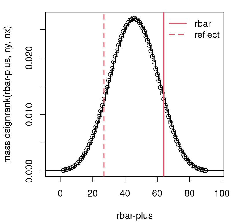
FIGURE 9.3: Exact \(\bar{R}^+\) sampling distribution for blood circulation example without ties.
The latter is used for \(p\)-value calculation. Since observed \(\bar{r}^+\)
is in the right tail, one must both provide lower.tail=FALSE and subtract
one from the statistic, because of the discrete nature of the distribution.
Alternatively, you may use the reflected statistic (unaltered) and work in the
left tail. Check your work with wilcox.test(..., paired=TRUE),
which is set up like t.test().
pval.exact <- 2*psignrank(rbarp - 1, n, lower.tail=FALSE)
pval.lib <- wilcox.test(y, x, paired=TRUE)$p.value
c(mc=pval.mc, exact=pval.exact,
  reflect=2*psignrank(2*Rbarp.mean-rbarp, n), lib=pval.lib)
## mc exact reflect lib
## 0.2155 0.2163 0.2163 0.2163Now on to the second example involving mental puzzles under physical fatigue. When there are ties, as there are in these data – and/or \(n\) is too large for solving SSPs (or for MC simulation) – the CLT may be used. For reasons that are not completely clear to me, it is common to use a different statistic with the CLT. It seems to me that it would be just as easy to work with positive signed ranks (9.6), but instead it’s preferred to use the sum of all signed ranks (9.3) with the CLT. (Note that Eq. (9.3) was developed in the context of unsigned ranks on a combined sample, but here I’m reinterpreting it for signed ranks on differences, \(d_i\), following Eq. (9.5).)
Clearly \(\mathbb{E}\{\bar{R}\} = 0\) since each rank is equally likely to be positive or negative under the null (9.2). Working out the variance isn’t much harder.
\[ \mathbb{V}\mathrm{ar}\{\bar{R}\} = \sum_{i=1}^n \mathbb{V}\mathrm{ar}\{R_i\} = \sum_{i=1}^n \mathbb{E}\{R_i^2\} - \mathbb{E}\{R_i\}^2 = \sum_{i=1}^n R_i^2 \]
The last step follows since \(\mathbb{E}\{R_i\} = 0\). Reducing from \(\mathbb{E}\{R_i^2\}\) to \(R_i^2\) is a bit of a slight-of-hand. The square obliterates the sign of the signed rank since \((-1)^2 = 1\). Since every rank is possible, but only one rank can be held by each of \(i=1,\dots,n\) at a time, it must be that all ranks are present when summing what to “expect” over all \(i\). The end result isn’t that helpful, though, since \(R_i\) are capitalized random variables. The best we can do is slot in observed \(r_i\). If there are no ties, then \(\sum_{i=1}^n i^2 = n(n+1)(2n + 1)/6\), a so-called pyramidal number. That could be helpful if your only calculating tool is pen-and-paper, like on an exam, where summing up lots of squares isn’t practical. (Our example has ties.)
Summarizing, we have
\[ Z = \frac{\bar{R}}{\sqrt{\sum_{i=1}^n r_i^2}} \sim \mathcal{N}(0, 1) \quad \mbox{ as } \quad n \rightarrow \infty. \]
Therefore, the following calculations provide an approximate \(p\)-value for fixed \(n\).
z <- sum(sr2)/sqrt(sum(sr2^2))
pval2.clt <- 2*pnorm(-abs(z))
c(mc=pval2.mc, mc.ties=pval2.mc.ties, clt=pval2.clt,
  lib=wilcox.test(y2, x2, paired=TRUE, exact=FALSE, correct=FALSE)$p.value)
## mc mc.ties clt lib
## 0.01614 0.01553 0.01851 0.01851This is definitely in the ballpark. Keep in mind everything that in the printout above is an approximation. None of these numbers leads to a different conclusion; not even close. All evidence points to fatigue impacting mental performance.
The calculations above omit a continuity correction (correct=FALSE). If
you wish to compare to correct=TRUE, make the following adjustment.
z.numer <- sum(sr2)
z <- (z.numer - sign(z.numer))/sqrt(sum(sr2^2))
c(2*pnorm(-abs(z)), wilcox.test(y2, x2, paired=TRUE, exact=FALSE)$p.value)
## [1] 0.02056 0.02056It’s not clear to me why adding \(\pm 1\) is required this time, whereas it was \(\pm \frac{1}{2}\) previously. I know that, as the author of this book, you’re looking to me to be an authority. But these things are the worst part about statistics, in my opinion. Off-by-a-half (or by one) issues can be a huge distraction to understanding the big picture in any subject. If something so small substantively changes the calculation in a statistical analysis, and ultimately affects big downstream decision-making, then the whole enterprise is flawed. Go back to the drawing board. Do a new/bigger experiment, and get less lost in the weeds of a Gaussian approximation. Or, use MC.
9.4 One sample non-P location
A signed ranks test can also be applied for a single sample, to test for a mean (or median, since the symmetry assumption makes those the same). Assume \(Y_1, \dots, Y_{n'} \stackrel{\mathrm{iid}}{\sim} F_Y\), for some symmetric \(F_Y\). Suppose you want to know if \(\mathbb{E}\{Y_i\} = \mu\) for some value of interest \(\mu\). Formally, the hypotheses are as in Eq. (9.2), except replace \(\mathbb{E}\{X\} = \mu\) everywhere. There is no \(X\) sample or \(F_X\).
The testing procedure is as in §9.3 except everywhere there’s an \(X_i\), replace with \(\mu\) instead. Just treat the data as \((\mu, y_1), \dots, (\mu, y_{n'})\) and push on. If any of the \(d_i = y_i - \mu = 0\), then discard that data point, and let \(n\) be the number of nonzero \(d_1, \dots, d_n\) that remain. There could still be ties in the ranks, etc., so everything else still applies.
Since this is pretty straightforward, I’m not going to cover all of the cases with examples. One should do. So here we go. Intelligence Quotient (IQ) tests are designed to produce scores that average around 100 with a standard deviation of 15, meaning that 95% of scores range from 70 to 130. Since IQ scores are whole numbers, a Gaussian assumption may not be appropriate although assuming a symmetric distribution may be reasonable. Scores quoted below come from teenagers in a certain small college town with affluent parents who might be overzealous micro-managers of their children’s education.
y <- c(95, 101, 100, 115, 105, 99, 101, 107, 120, 100, 98, 77, 89, 121,
  102, 97, 106, 111, 101, 107, 102, 88, 112, 128)
More than 70% of these scores are above 100, so you might be inclined to think that kids in this town are exceptionally smart based on this sample. That’s a statistic, but it’s not statistical inference. Can we reject the hippopotamus that these data were generated from a distribution with \(\mathbb{E}\{Y\} = 100\)?
Rather than re-code everything, I prefer to simply assign x <- mu and
then cut-and-paste.
x <- 100              ## E(Y) = mu = 100
nprime <- length(y)
d <- y - x
d <- d[d != 0]
n <- length(d)
r <- rank(abs(d))
sr <- r*sign(d)
rbarp <- sum(sr[sr > 0])
c(nprime=nprime, n=n, u=length(unique(r)), rbarp=rbarp)
## nprime n u rbarp
## 24 22 13 175It looks like two zeros were removed, and there are lots of ties in the ranks.
##
## 2 3 4
## 4 1 1
Here’s a single MC that entertains a sampling distribution for \(\bar{R}^+\) in two situations: ignoring ties, and mimicking them stochastically.
Rubarps <- Rtbarps <- rep(NA, N)
ranks <- 1:n                                      ## ranks without ties
for(i in 1:N) {

  ## deal with ties
  rd4 <- rank.ties(ranks, 1, 4)                   ## 1 degree-4 tie
  rd3 <- rank.ties(rd4$ranks, 1, 3, rd4$uniq)     ## 1 degree-3 tie
  rd2 <- rank.ties(rd3$ranks, 4, 2, rd3$uniq)     ## 4 degree-2 ties

  ## permute
  perm <- sample(ranks)                           ## shared permutation
  Rts <- rd2$ranks[perm]
  Rus <- ranks[perm]                              ## permute unique ranks

  ## signs
  signs <- sample(c(-1, 1), n, replace=TRUE)      ## shared random signs
  SRts <- Rts*signs
  SRus <- Rus*signs

  ## final statistic
  Rtbarps[i] <- sum(SRts[signs > 0])              ## rest as usual
  Rubarps[i] <- sum(SRus[signs > 0])

}
As you can see below, the \(p\)-values aren’t much different. There is not enough evidence to reject the null hypothesis. Over-parented children in this small town aren’t exceptionally smart.
## ignore    ack
## 0.1191 0.1169
Here are calculations doing things the math way. First, ignoring the
presence of ties, and performing calculations using closed-form calculations
via SSP. (There seems to be no way to force the library function
wilcox.test to use the exact calculation in the presence of ties. If there
are ties, then it spits out a warning and uses the CLT (exact=FALSE)
anyways.)
##  exact
## 0.1207
Finally, here is a version using a CLT approximation with continuity correction, first by hand and then with the library.
z.numer <- sum(sr)
z <- (z.numer - sign(z.numer))/sqrt(sum(sr^2))
c(clt=2*pnorm(-abs(z)), lib=wilcox.test(y, mu=100, exact=FALSE)$p.value)
## clt lib
## 0.1187 0.1187It’s pretty much the same outcome any way you slice it. And that’s lots of cutting-and-pasting. Perhaps it would make sense to write our own library function before jumping into your own analyses. Guess what’s coming next?
9.5 Homework exercises
These exercises help gain experience with Wilcoxon rank sum and signed rank tests. There are no math questions this time, all coding and/or data analysis. Most involve new data/problems, however many questions on \(t\)-tests from previous chapters (e.g., §2.6 and §5.4) offer good non-P practice. Don’t forget to try each test multiple ways, e.g., via MC or math as appropriate.
Do these problems with your own code, or code from this book. Unless stated explicitly otherwise, avoid use of libraries in your solutions.
#1: Subset sum for signed ranks
Follow the template provided for dranks and pranks in
rank_ties.R (via
§B.3), which is for rank sums, to provide a similar
capability for signed ranks. That is, appropriate the SSP solver from
those subroutines for working with signed ranks instead. You may check your
work against dsignrank and psignrank. Maybe call your version dsranks
and psranks.
#2: More stochasticity in ties
This one is a bit of a challenge problem. The (possibly) daisy-chained
rank.ties calls from this chapter mimic tie-degrees that are present in
observed ranks. Add flexibility to this by instead allowing the tying degree,
and the number of ties for each degree, to follow Poisson distributions.
Specifically, take the maximal tie degree as \(D \sim \mathrm{Pois}(\lambda_d)\).
Given \(D = d\), take the number of ties as \(T_1, \dots, T_d
\stackrel{\mathrm{iid}}{\sim} \mathrm{Pois}(\lambda_t)\). Generate new \(D\) and
\(\{T_j\}_{j=1}^d\) in each MC iteration.
You’ll still need to use rank.ties to find these ties for each degree, and
don’t forget to daisy chain from largest to smallest. Be careful not to ask for
too many, and of too-high a degree, for small \(n\), or it’ll break. That means
small \(\lambda_d\) and \(\lambda_t\), like \(\lambda_d = \lambda_t \leq 2\).
#3: monty.wilcoxon for one- and two-samples
Write a library function, inspired by monty.t from
§2.6 and §5.4, that covers all
variations of Wilcoxon tests. This includes two-sample, paired and unpaired,
and one-sample tests; MC, closed-form exact and CLT versions; special
considerations for ties (e.g., using rank.ties and optionally your solution
to #2), and warnings as needed when your user makes ill-advised choices. You
may use pwilcox or pranks and psignrank as desired, and pnorm as
usual. Support optional visuals.
Hint: many of the following questions are easier after this one is squared away. (You should be getting the hang of this by now.)
#4: Your brain on artificial intelligence
A team of neuroscientists recruited thirty participants for a study on the effects of artificial intelligence (AI) on memory. Each participant was asked to write an essay on a topic of interest to them. Before writing these essays, participants were randomly assigned to one of two groups. One, the control group, was asked to use a computer terminal (connected to the internet), but with all AI functionality locked out. The other, the AI group, had access to an ordinary terminal without restrictions and were encouraged to use AI. Later, each participant was asked to recall passages about their essays. Their accuracy in recollection exercises was assigned a score from 0 to 100. Those are provided below.
control <- c(72, 94, 72, 93, 72, 91, 63, 52, 84, 59, 70, 66, 98, 91, 71)
AI <- c(53, 52, 83, 81, 63, 71, 50, 86, 43, 77, 49, 63, 57, 41, 55)
What do you think? Does AI have an effect on the average recall score?
#5: Zoom learning
Two sections of the same statistics class, led by the same instructor, were
offered at VT one semester. Both classes were completely in sync: same
lectures, homework, exams, etc. The only differences were the students and the
official mode of instruction. One mode was “Zoom”, and the other was
“classic” in-person delivery. Students were even invited to attend classes,
and take exams, outside their registered modality (zoom or classic),
although anecdotally students rarely swapped modes. Final class percentages,
combining all homeworks and exams, are provided by
classmode.RData on the book webpage.
Is there a difference in mean scores for students across these two modalities?
#6: Non-P ROI
Refer back to roi$company and roi$industry from §2.5. Recall that these data are available as roi.RData on the book webpage.
Based on a non-P analysis, does there seem to be any difference in mean ROI between companies that use the IT product in question and the industry at large? You may have studied this parametrically in §5.4, and via bootstrap and permutation tests in Chapter 8.
#7: Identical twin multivitamin study
Twin studies are popular as a means of mitigating subject variability, among other (especially) genetic factors, in treatment–control trials (a.k.a., A/B tests). Twenty pairs of twins were recruited for a study of the effectiveness of an over-the-counter multivitamin on the immune system. In each pair of twins, one was randomly selected to take the multivitamin, and the other a placebo. After 30 days all participants had their blood drawn in order to measure T-cell counts, in cells per cubic millimeter of blood. These numbers are recorded below.
placebo <- c(1002, 517, 1100, 790, 1333, 787, 803, 720, 1243, 850, 696,
  713, 769, 556, 873, 563, 922, 660, 1401, 810)
multivit <- c(956, 693, 1044, 920, 1258, 873, 883, 1033, 1476, 940, 947,
  463, 678, 717, 775, 723, 1033, 715, 1245, 798)
What do you think? Does this particular multivitamin boost the immune system?
#8: Non-P paired ROI
Return to roip.csv on the book webage, which pairs company and industry ROI row-wise.
Perform a non-P analysis to determine if roip$company and roip$industry
have different means. You may have studied this parametrically in
§5.4.
#9: Benzene conversions
Nandi et al. (2002) studied benzene conversions, measured in mole percent, for twenty-four different benzenehydroxylation reactions.
convs <- c(80.8, 59.4, 19, 30.1, 30.1, 81.2, 28.8, 40, 67.8, 26.8, 63, 80.8,
  40.0, 30.3, 41, 38.1, 81.2, 52.3, 36.2, 36.2, 33.4, 19, 9.1, 30.1)
Industrial application requires that mean conversions be 30 mole percent, or greater. What do you think?
References
ANSM5: Functions and Data for the Book “Applied Nonparametric Statistical Methods,” 5th Edition. https://doi.org/10.32614/CRAN.package.ANSM5.
In fact, the null (9.2) says \(\mathbb{E}\{Y\} = \mathbb{E}\{X\}\) which is weaker, because the Wilcoxon rank sum test “targets” means. But it’s ok to strengthen the null. It is certainly the case that if \(F_Y = F_X\) then \(\mathbb{E}\{Y\} = \mathbb{E}\{X\}\).↩︎
If you’re curious,
wilcox.testresides insrc/library/stats/R.↩︎It is technically known as the signed rank test. I’ve made it plural because I like it better. No rank makes sense in a vacuum, i.e., without other ranks.↩︎