Chapter 6 Analysis of variance

This chapter lumps two things together which are actually quite distinct. One is tests that focus on variance, like \(\sigma^2\) in a Gaussian sample. We’ll do this for one sample and for two samples. My own feeling is that this has somewhat limited utility compared to things we’ve covered up until this point. It certainly can be useful, like to check if one process is more variable – more wobbly in its behavior – than another. But variance is often a second-order concern. (It’s already a second moment.)

The second thing is eponymous in the title: analysis of variance (ANOVA). ANOVA is super useful. The trouble is, it’s not really about variance. It’s about means. True, you do analyze variance(s), but as a means to an end for means. You don’t use analysis of variance to test for variance. I prefer to think of it as a pooled-variance extension of the two-sample Gaussian test of §5.2, but to three or more samples. (You can also do it for two samples, but it doesn’t make sense for a single sample.)

Statisticians are notoriously bad at naming things. You might even argue that the choice of the word “statistics” was a mistake. Too much of a mouthful. Apologies to my Greek friends. Another great example is regression, which we’ll cover in Chapter 7. Regression is a super important and exciting topic with a terrible name. No parent wants to hear that their child is regressing in school.

Machine learning (ML) researchers are much better at naming. Instead of “logistic regression”, or “logit regression” for short (those are stats terms), ML has the “perceptron”. I don’t actually cover either topic in this book, though they are both cool and important (maybe in volume two). I’m just trying to make a point here, and there are lots of other great examples. In Chapter 5 I said that two-sample \(t\)-testing is a form of A/B testing, which comes from ML. I don’t think there is any direct analog of ANOVA in the ML world, but if there were, I think they would call it an “alphabet test”, because it’s like “A/B/C/D/… testing”. Better right?

So why did I lump these two topics together? One reason is that I wanted to cover both, but two separate chapters would have been rather thin. I’ll lump these two topics together for the same reason when we treat their nonparametric cousins in Chapter 11. The second reason is everyone thinks ANOVA is about variance, and therefore is right at home alongside other variance tests. That might be wrong, but it lets me spin a tidy yarn that I hope you won’t forget.

6.1 One sample

This will be quick, so I’m just going to jump right in. Here the model is the same as in §2.1, but I’ll repeat it below for convenience.

\[\begin{equation} \mbox{Model:} \quad\quad Y_1, \dots, Y_n \stackrel{\mathrm{iid}}{\sim} \mathcal{N}(\mu, \sigma^2) \tag{6.1} \end{equation}\]

This time interest lies in \(\sigma^2\) not \(\mu\). Suppose there were some value \(\sigma_0^2\) that you were wondering about. You could pose the following competing hypotheses.

\[\begin{align*} \mathcal{H}_0 &: \sigma^2 = \textstyle \sigma_0^2 && \mbox{null hypothesis (``what if'')} \\ \mathcal{H}_1 &: \sigma^2 \ne \sigma_0^2 && \mbox{alternative hypothesis} \end{align*}\]

The value of \(\mu\) isn’t pinned down by the hypotheses. Any value will work for carrying out the test by Monte Carlo (MC). However, the usual statistic that’s used for variance, \(s^2\) from Eq. (3.6) has an implicit \(\bar{y}\) built in.

To have something concrete for calculations, consider the following example. The owner of a major ice cream franchise, understandably, wants to control the variability of the size of ice cream scoops in his store. He’s concerned, in particular, about one goofball employee whose carefree attitude would seem to be at odds with consistency in any aspect of his life. He recruits sixteen confederate customers who order ice cream at the shop, and who are served by this particular employee. Their scoops are weighed and the results are below.

y <- c(4.0, 5.5, 4.9, 3.8, 4.3, 4.4, 5.1, 4.1, 4.0, 3.0, 3.7, 3.4, 3.6,
  3.0, 3.5, 4.0)
n <- length(y)
s2 <- var(y)

Once you’ve calculated \(s^2\) and extracted \(n\), you don’t need the individual \(y\)-values anymore. These quantities comprise sufficient information about the sample for the purposes of inference.

According to Google, a scoop of ice cream is typically around 4 oz. During training, all employees were taught how to scoop ice cream such that scoops were between 3 and 5 oz, 95% of the time. In other words, with variance \(\sigma^2 = 0.5^2\).

mu <- 4
sigma2 <- 0.5^2

The franchise owner hired us as statistical consultants. What can we tell him about how these data related to those targets, in particular as regards \(\sigma^2\)?

One-sample variance test by MC

The code below takes \(n\)-sized samples from the null hippopotamus (\(\sigma^2 = 0.5^2\)) and calculates their variance, repeatedly in a MC fashion. The value taken for \(\mu\) is as specified above, but again any \(\mu\) will do.

N <- 100000
S2s <- rep(NA, N) 
for(i in 1:N) {
  Ys <- rnorm(n, mu, sqrt(sigma2))
  s2s <- var(Ys)
  S2s[i] <- s2s
}

Figure 6.1 offers a visual of the empirical sampling distribution of those variances with the value of \(s^2\) from the data (and its reflection) overlayed. That observed statistic is out in the tails, but not so far out. It’s a close call.

hist(S2s, main="", xlim=range(c(s2, S2s)))
abline(v=c(s2, quantile(S2s, mean(S2s > s2))), lty=1:2, col=2, lwd=2)
legend("topright", c("s2", "reflect"), col=2, lty=1:2, lwd=2, bty="n")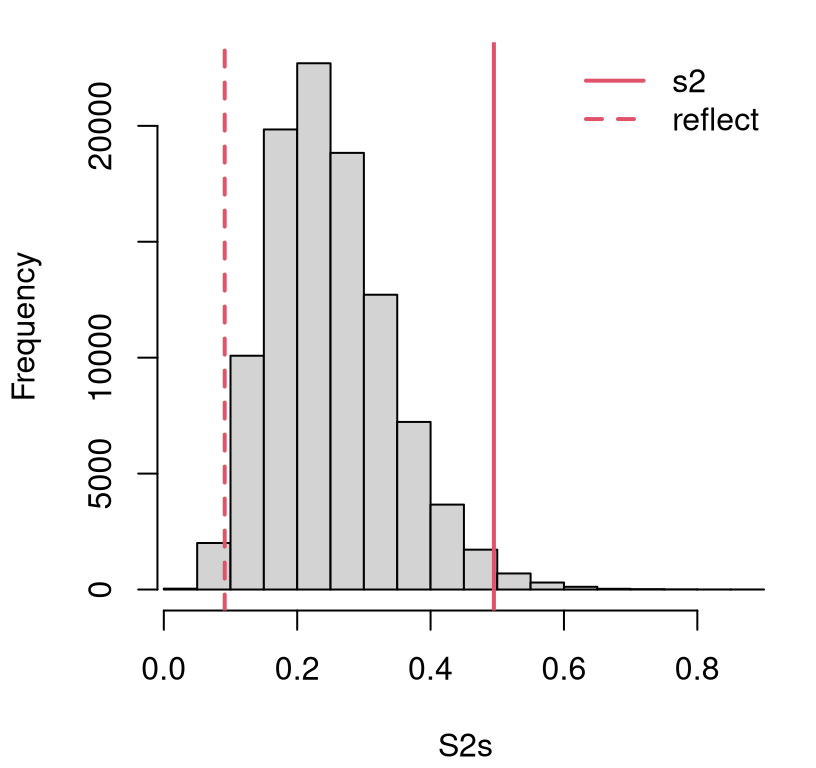

FIGURE 6.1: Histogram of sampled variances under \(\mathcal{H}_0\) compared to the observed variance and its reflection.

To help quantify the outcome of the test, a \(p\)-value may be calculated as follows.

pval.mc <- 2*mean(S2s > s2)
pval.mc

## [1] 0.02572

This is comfortably below our usual 5% threshold. So we might decide to reject the null hypothesis and conclude that this particular employee’s scooping is more variable than his boss would like. Yet I recommend against firing the poor bloke, yet. The situation is more nuanced than I have described. But before we get to that, how would you do this the old-school math way?

One-sample variance test by math

Recall from Chapter 3 that sums of Gaussian squares have a (scaled) \(\chi^2\) distribution. Those sums of squares are exactly what we simulated above, under \(\mathcal{H}_0\). In particular, Eq. (3.16) provides that

\[ V \equiv \frac{(n-1)S^2}{\sigma^2} \sim \chi_{n-1}^2. \]

Notice how that equation relays both the test statistic, \(v = \frac{(n-1)s^2}{\sigma^2}\) using observed data values and for any \(\sigma^2\) of interest (provided by \(\mathcal{H}_0\)), and its sampling distribution \(V \sim \chi_{n-1}^2\).

v <- s2*(n - 1)/sigma2

Quick digression on notation. I chose the letter \(V\) because the quantity in question is a (scaled) variance. Many texts use a generic \(t\) for “test” statistics, but I think that’s confusing because it clashes with the statistic involved \(t\)-tests, which have a \(t_\nu\) distribution. Variances, and residual sums of squares more widely, usually have a \(\chi^2_\nu\) distribution.

Alright, back to our analysis. The visual for the statistic \(v\) and its distribution, provided in Figure 6.2, is similar to the empirical distribution of Figure 6.1, except scaled by \((n-1)/\sigma^2\).

x <- seq(0, 3*n, length(1000))
plot(x, dchisq(x, n-1), type="l", lwd=2, main="")
abline(v=c(v, qchisq(pchisq(v, n - 1, lower.tail=FALSE), n - 1)), 
  lty=1:2, col=2, lwd=2)
legend("topright", c("v", "reflect"), lty=1:2, col=2, lwd=2, bty="n")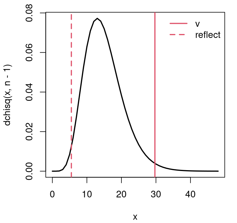

FIGURE 6.2: Sampling distribution and observed statistic for one-sample variance test.

We may calculate a \(p\)-value by integrating into the two tails as follows. Remember to be careful to get the direction of the tail right with the lower.tail argument. This could change depending on what side of the distribution your statistic is on. With this two-tailed test, I’m presuming a reflected value lying at the opposite quantile, as shown in the figure. This is why I can get away with multiplying by 2.

pval.math <- 2*pchisq(v, n - 1, lower.tail=FALSE) 
c(mc=pval.mc, math=pval.math)

##      mc    math 
## 0.02572 0.02612

That \(p\)-value is in close agreement with our MC calculation earlier. There’s no variance test built-into R; however, I found one in the EnvStats package on CRAN (Millard 2013).

library(EnvStats)   ## you man need to install.packages("EnvStats") first
varTest(y, sigma.squared=sigma2)$p.value

## [1] 0.02612

The same \(p\)-value we calculated by hand above.

Confidence intervals

Before turning to two-sample tests, I want to make a quick note about confidence intervals (CIs). Remember, once you know the sampling distribution – whether empirically via MC or via math – it’s easy to form a CI. In our current context, that means one of two things. Either replace estimated \(s^2\) with \(\sigma^2\) in the MC. (I’ve left that one for you as a homework exercise in §6.5.) Or, if you prefer the math way, follow the outline in §3.3. First find quantiles of the distribution, in this case \(\chi^2_{n-1}\). Then undo the re-scaling to solve of \(\sigma^2\) on both sides of the inequality.

\[\begin{align*} 1 - \alpha = \mathbb{P}(q_{\alpha/2} < z < q_{1 - \alpha/2}) &= \mathbb{P}\left(q_{\alpha/2} < \frac{(n-1)s^2}{\sigma^2} < q_{1 - \alpha/2}\right) \\ &= \mathbb{P}\left(\frac{s^2(n-1)}{q_{1-\alpha/2}} < \sigma^2 < \frac{s^2(n-1)}{q_{1\alpha/2}}\right) \end{align*}\]

Don’t forget to flip around your inequalities when you divide all sides by \(\sigma^2\) to put it in the numerator. Here are those calculations in code.

q <- qchisq(c(0.025, 0.975), n - 1)
CI.math <- s2*(n - 1)/rev(q)            ## rev to flip inequalities

Here it comes with the library-based calculation for comparison.

CI.lib <- as.numeric(varTest(y, sigma.squared=sigma2)$conf.int)
rbind(math=CI.math, lib=CI.lib)

##        [,1]  [,2]
## math 0.2701 1.186
## lib  0.2701 1.186

Those are identical.

I know I said, on multiple occasions, the math way to get a CI is \(\mathrm{est} \pm q\times \mathrm{se}\). (Use \(q = 2\) for an approximate 95% interval). That’s only if we have “\(\mathrm{est}\)” and “\(\mathrm{se}\)” and are willing to make a Gaussian approximation. We have the exact sampling distribution in this instance, so no need to approximate. But if you insist, check this out. Eq. (4.9) gives the following asymptotic approximation by way of the MLE for \(\sigma^2\).

\[ \hat{\sigma}^2 \sim \mathcal{N}(\sigma^2, 2\sigma^4/n) \quad \mbox{ as } \quad n \rightarrow \infty. \]

Therein lies the standard error we require: \(\mathrm{se} = \sqrt{2(\hat{\sigma}^2)^2/n}\), after plugging in \(\hat{\sigma}^2\) for \(\sigma^2\) following the weak law of large numbers (WLLN).

s2hat <- s2*(n - 1)/n
se <- sqrt(2*s2hat^2/n)
CI.asy <- s2hat + c(-2, 2)*se
CI.asy

## [1] 0.1359 0.7921

This isn’t a great approximation since \(n = 16 \ll \infty\). You have to be particularly careful with approximate Gaussian CIs near zero. Both ends of the interval calculated above fit this description; the left one especially. In that situation, there’s a non-negligible amount of density on negative values, but variances can’t be negative. When the actual (\(\chi^2_{n-1}\)) sampling distribution is substantially skewed – see Figure 6.2 – an approximately Gaussian-based CI estimate is biased toward zero, and is too small to have appropriate nominal coverage.

This is, in my opinion, all really cumbersome compared to the MC version which involves essentially one replacement: sigma2 <- s2. You may draw your own conclusion after trying for yourself in homework exercises. Coding effort aside, it bears repeating … When you must approximate numerically, MC trumps Gaussian asymptotics. The only exception might be when \(n\) is really large.

6.2 Two samples

Suppose I told you that the last seven scoops were not of ice cream, but instead sorbet. Sorbet is water-based and generally weighs less than dairy-based ice cream, per unit volume. So if our beleaguered employee is using the same scooper and technique, and producing the same volume of ice cream each time, it stands to reason that his ice cream scoops would weigh more than his sorbet ones, and also possibly have different variance.

For now, I plan to keep focus on variance. Means are next in §6.3. Here is the situation, with \(y\)’s now capturing ice cream scoops, and \(x\)’s for sorbet.

x <- y[10:16]       ## sorbet
s2x <- var(x)
nx <- length(x)
y <- y[1:9]         ## ice cream
ny <- length(y)
s2y <- var(y)

It can be helpful to visualize these data just to fix ideas. See Figure 6.3. There’s a clear location shift, but the question of variance is more subtle. Observe how the spread of red dots (\(x\): sorbet) is a little narrower than the black open circles (\(y\): ice cream). Is that difference statistically significant?

plot(y, abs(rnorm(ny, 0, 0.1)), ylim=c(-0.5, 2.25), 
  xlim=c(range(y, x)), xlab="weights", ylab="", yaxt="n", bty="n")
points(x, abs(rnorm(nx, 0.75, 0.1)), col=2, pch=19)
legend("top", c("ice cream", "sorbet"), col=1:2, pch=c(21, 19), 
  bty="n", horiz=TRUE)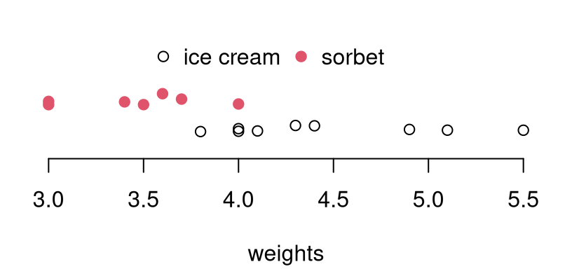

FIGURE 6.3: Comparing ice cream and sorbet weight data. Vertical jitter is added to help visualize duplicates.

We wish to determine if this employee’s scoops of ice cream have the same weight variability as his scoops of sorbet. (Not the same mean.) The modeling setup is the same as Eq. (5.5) in §5.2, but I’ll repeat it here for convenience.

\[ \begin{aligned} \mbox{Model:} && Y_1, \dots, Y_{n_y} &\stackrel{\mathrm{iid}}{\sim} \mathcal{N}(\mu_y, \sigma_y^2) & & \mbox{and} & X_1, \dots, X_{n_x} &\stackrel{\mathrm{iid}}{\sim} \mathcal{N}(\mu_x, \sigma_x^2) \end{aligned} \]

Now, the competing hypotheses of interest, characterizing the “want to know”, are different.

\[\begin{align*} \mathcal{H}_0 &: \sigma^2_y = \sigma^2_x && \mbox{null hypothesis (``what if'')} \\ \mathcal{H}_1 &: \sigma^2_y \ne \sigma^2_x && \mbox{alternative hypothesis} \end{align*}\]

When inspecting means in §5.2 we pivoted from \(\mu_y = \mu_x\) to \(\mu_y - \mu_x = 0\). We might do that here too, but variances must always be positive, and so it’s awkward to take differences because they might go negative. Instead, it’s more natural to inspect ratios: \(\sigma_y^2/\sigma_x^2 = 1\). There’s another good reason for preferring a ratio over a difference that has to do with the math way of conducting the test, which I’ll get to soon. A sensible test statistic is therefore

\[ f = s_y^2/s_x^2, \]

or vice versa: \(f = s_x^2/s_y^2\); it doesn’t matter much, although I’ll tell you that it’s customary to put the larger one (in this case \(s_y^2\)) in the numerator. The reason for the letter \(f\), and for this convention, will become apparent later. For now, yes, you guessed it: \(F\) is for Fisher.

f <- s2y/s2x
f

## [1] 2.542

This value is not, in isolation, very informative. Apparently, the variance of this employee’s ice cream scoops is \(2.54 \times\) larger than sorbet. One problem with that is that humans are bad at interpreting things in units of squared quantities. Back on the scale of standard deviations, which have units of ounces, it’s more like 1.59\(\times\) more. But more importantly, we don’t know what sorts of \(F\)-values are likely under \(\mathcal{H}_0\). We, as yet, have nothing to compare this \(f\) statistic to.

Two-sample variance test by MC

R code below samples from the empirical null distribution of \(F\), the random analog of \(f\). As in §5.2, it doesn’t matter what values of \(\mu_x\) and \(\mu_y\) are used, and they may even be the same: \(\mu \equiv \mu_y = \mu_x\). The same is true for \(\sigma^2 \equiv \sigma^2_y = \sigma_x^2\), except that they must be the same because \(\mathcal{H}_0\) says so. Below, I arbitrarily stick with mu defined earlier, and keep it simple with \(\sigma^2 = 1\).

sigma2 <- 1
Fs <- rep(NA, N)
for(i in 1:N) {
  Ys <- rnorm(ny, mu, sqrt(sigma2))
  Xs <- rnorm(nx, mu, sqrt(sigma2))
  s2ys <- var(Ys)
  s2xs <- var(Xs)
  Fs[i] <- s2ys/s2xs
}

When you think about this setup a little, you realize that the only quantities which change from one analysis to the next are \(n_y\) and \(n_x\). Nothing else matters. Interesting, right? Figure 6.4 shows the empirical sampling distribution of \(F\) based on \(n_y=9\) and \(n_x = 7\) from the scooping experiment.

hist(Fs[Fs < 8], main="", xlim=range(c(0,8)))  ## focus histogram near 0
abline(v=c(f, quantile(Fs, mean(Fs > f))), lty=1:2, col=2, lwd=2)
legend("topright", c("f", "reflect"), col=2, lty=1:2, lwd=2, bty="n")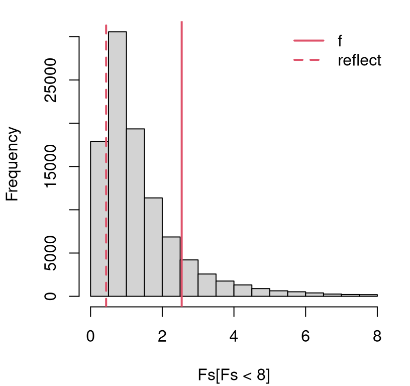

FIGURE 6.4: Empirical sampling distribution of \(F\) from the ice cream and sorbet scooping experiment.

The sampling distribution of these \(F\)-values can be quite heavily right-tailed. This is the reason for Fs[Fs < 8], focusing our attention near the origin. Without that, the \(x\)-axis of the histogram would extend out \(\sim 50\times\) longer and, partly as a consequence, histogram binning would have low resolution. I’ll give another reason why 8 is a good choice later.

summary(Fs)

##     Min.  1st Qu.   Median     Mean  3rd Qu.     Max. 
##   0.0302   0.6066   1.0328   1.5041   1.7798 458.0424

It’s pretty clear from Figure 6.4 that we do not have enough evidence to reject the null hypothesis. Putting the larger of \(s_y^2\) and \(s_x^2\) in the numerator, so that \(f = s_y^2 / s_x^2 > 1\), ensures that the statistic is also in the right tail. This leads to a more streamlined two-tailed \(p\)-value calculation because the inequality is always “>”.

pval.mc <- 2*mean(Fs > f)
pval.mc

## [1] 0.2713

It turns out that, across these two types of tasty frozen desserts, this otherwise goofball employee in fact has a good, consistent scooping hand. The real issue is that one weight for all ice creams, sorbets, gelatos, fat-free ice creams, etc., might not be appropriate as a measure for quality control.

Two-sample variance test by math

By two applications of analogous one-sample results, ultimately tracing things back to Eq. (3.16),

\[\begin{equation} S_y^2 \sim \frac{\chi_{n_y - 1}^2 \sigma_y^2}{n_y - 1} \quad \mbox{ and } \quad S_x^2 \sim \frac{\chi_{n_x - 1}^2 \sigma_x^2}{n_x - 1}. \tag{6.2} \end{equation}\]

When studying their ratio, there is some cancellation under the null hypothesis, giving \(\sigma_y^2 = \sigma_x^2\).

\[\begin{equation} F = \frac{S_y^2}{S_x^2} \sim \frac{\chi_{n_y - 1}^2/(n_y - 1)}{\chi_{n_x - 1}^2/(n_x - 1)} \tag{6.3} \end{equation}\]

Ronald Fisher may have been the first to extensively study ratios of normalized \(\chi^2\) random variables, but George Snedecor is credited with characterizing a closed form for their distribution. Snedecor graciously named it after Fisher, and it is now known as the \(F\) distribution. An \(F\) distribution has two parameters, affectionately named the numerator and denominator degrees of freedom (DoF), respectively, which come from the \(\chi^2\) statistics located in those positions of the ratio.

Summarizing, we have

\[\begin{equation} F \sim F_{n_y - 1, n_x - 1}. \tag{6.4} \end{equation}\]

It’s a little confusing to have a random variable, \(F\), take on the same name and capitalization as \(F_{n_y - 1, n_x - 1}\). Don’t shoot the messenger. I’m not going to quote much else about the distribution, which you can anyways find on Wikipedia, except the following two nuggets. It is a distribution over positive quantities, because it involves ratios of positive (squared) values, and so it has a right skew. Pretty much for any DoF arguments bigger than a handful (\(n_x, n_y > 4\) or so), 95% of the cumulative density lies to the left of four. This is similar to 95% of a standard Gaussian or \(t_\nu\) distribution being in \([-2, 2]\). (And it’s not a coincidence that \(2^2 = 4\). More on this in §6.4.) So there’s a nice rule of thumb for \(F\)-tests, like for \(t\)- and \(z\)-tests. You will likely reject at the 5% level if \(f > 4\). It also means there’s rarely much cause to plot the density much beyond four. I doubled that to eight in Figure 6.4, and again momentarily in Figure 6.5.

fgrid <- seq(0, 8, length=1000)
plot(fgrid, df(fgrid, ny - 1, nx - 1), type="l", lwd=2, main="")
abline(v=c(f, qf(pf(f, ny - 1, nx - 1, lower.tail=FALSE), ny - 1, nx - 1)), 
  lty=1:2, col=2, lwd=2)
legend("topright", c("f", "reflect"), lty=1:2, col=2, lwd=2, bty="n")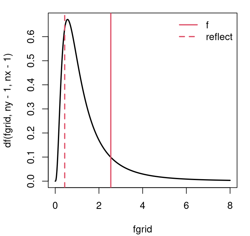

FIGURE 6.5: \(F\) distribution and observed \(f\) statistic for the ice cream and sorbet test.

This view is similar to Figure 6.4, and therefore so is the \(p\)-value.

pval.f <- 2*pf(f, ny - 1, nx - 1, lower.tail=FALSE)
c(mc=pval.mc, f=pval.f)

##     mc      f 
## 0.2713 0.2719

There’s a built-in library function for two-sample variance tests in R, and it gives the same answer as our by-hand calculation.

var.test(y, x)$p.value

## [1] 0.2719

---

You can build a CI for a ratio of variances, but I’m not going to bore you with that, or even leave it to you as a homework exercise. You’re welcome. If you’re really curious, just follow the example(s) provided by the one-sample test(s).

A two-sample variance uses an \(f\) statistic under an \(F\) distribution, so you might think you’re doing an \(F\)-test. Sort of, but that’s not what most people mean when they say they’re doing an \(F\)-test. They’re thinking of ANOVA, which is what I’m about to cover next (§6.3), or they’re thinking of a (multiple) linear model selection test which is the subject of §13.5. And those two things are related.

6.3 ANOVA

Alright, suppose we had one more set of scoops, this time for servings of fat-free ice cream. These numbers are stored in w below.

w <- c(3.5, 3.4, 3.7, 3.4, 3.9, 4.2, 4.0, 4.0, 3.8, 3.8)

But I want to reorganize things a little, because I want to get away from \(y\), \(x\), and \(w\) notation. That’s not scalable. I need a data structure that can have any number of categories: \(1, 2, 3, \dots, m\) for arbitrary \(m\). The first way is as a list in R.

ylist <- list(cream=y, sorbet=x, fatfree=w)
ylist

## $cream
## [1] 4.0 5.5 4.9 3.8 4.3 4.4 5.1 4.1 4.0
## 
## $sorbet
## [1] 3.0 3.7 3.4 3.6 3.0 3.5 4.0
## 
## $fatfree
##  [1] 3.5 3.4 3.7 3.4 3.9 4.2 4.0 4.0 3.8 3.8

Having a list makes it easy to extract information by “applying” a function over entries in the list, like using length with sapply.

nj <- sapply(ylist, length)
m <- length(nj)
n <- sum(nj)
nj

##   cream  sorbet fatfree 
##       9       7      10

I’ll explain those variables momentarily, and their names will make more sense in due course. R has many automations built in for different (common) statistical data types. Another way to represent similar information in R is as a data.frame.

ydf <- data.frame(weight=unlist(ylist), type=factor(rep(1:m, nj)))

I’m not going to print that one to the page because it takes up too much space. I encourage you to do that on your own. Many things that sapply can do for list objects, tapply accomplish on a data.frame. I’ll show you later. Figure 6.6 demonstrates how both representations can be useful for visualization, with actual observations overlaid on a “box-and-whisker” summary (a.k.a., “boxplot”) of those values.

boxplot(ylist, border=1:3, ylab="weight")
jit <- rnorm(n, 0, 0.05)
points(as.numeric(ydf$type) + jit, ydf$weight, pch=19, 
  col=ydf$type, cex=0.75)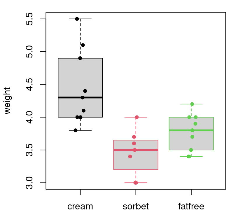

FIGURE 6.6: Visualizing the full ice cream scoop weight data set, with horizontal jitter.

Boxplots are my go-to for exploratory analysis of so-called “grouped” data in R. After plain plot, I use boxplot more than any visualization function in R. Let me encourage you read up on boxplots so you can see how the gray rectangle (the “box”) and their interval extension (“whiskers”) are defined. Be careful, the thin black line in the middle is the sample median, not the average. Sometimes, a small number of outliers are shown as open circles beyond the whiskers, but there aren’t any data points meeting the criteria for that in the scoop data.

Depending on what you want to do, a list or data.frame representation of grouped data might be more handy. Both are flexible enough to hold the type of data we’re considering here. Although there are only \(m = 3\) groups in the scoop data, what I’m about to show you applies for arbitrary \(m\), and any amount of data in each group, represented by nj in the code. Both the math and the code are intended to be generic enough for a wide class of problems/data of this type.

Now, as I said in the preamble to this chapter, an analysis of variance (ANOVA) is really a study of means. I will show you how to use ANOVA to tell if the scooping weights of Figure 6.6 really come from populations with different means, that is, whether this employee (using a standard scooper) is making scoops of different weights, on average, depending on what type of frozen treat is being scooped. Informally, that’s our “want to know”. More generically, we wish to tell if a grouping variable – in this case, frozen scooped treat type – is a statistically significant location factor in the variability of the \(y\)-values – in this case, weights.

Notice how I’m being careful with my words in italics. In ANOVA we do study variability (the V in ANOVA). Still, I think it’s a misnomer because means is what we really want to know about. That’ll become more clear when I lay out the modeling apparatus and hypotheses.

ANOVA model, hypotheses and statistic

Since the number of groups, \(m\), is arbitrary, we’ll have to be a little more nimble with notation. Don’t be frightened by the double-subscript indices. When you ponder it, they help with compactness. The model behind ANOVA is as follows.

\[\begin{equation} \mbox{Model:} \quad\quad Y_{ij} \stackrel{\mathrm{iid}}{\sim} \mathcal{N}(\mu_j, \sigma^2) \quad\quad i=1,\dots,n_j \ \mbox{ and } \ j=1,\dots,m \tag{6.5} \end{equation}\]

Similarly, record observations as \(y_{ij}\) over the same indices. You can say that \(y_{ij}\) stores the \(i^\mathrm{th}\) observation in the \(j^\mathrm{th}\) group. As shorthand, it helps to extract quantities like

\[ y_{\cdot j} \equiv y_{1,j}, \dots, y_{n_j, j}, \]

to refer to a whole collection of data values in a particular (say \(j^\mathrm{th}\)) group.

An important thing to notice is that variance \(\sigma^2\) doesn’t have any subscripts, but means \(\mu_j\) do. Each group has its own mean, but they all share a common variance. So Eq. (6.5) nests the pooled setup of §5.2 in the \(m=2\) case. In that context, we might rewrite the \(j=1\) group as \(y_1,\dots, y_{n_y}\) with \(n_y \equiv n_1\) and the \(j=2\) group as \(x_1,\dots, x_{n_x}\) with \(n_x \equiv n_2\).

That’s the ANOVA model. An ANOVA system of competing hypotheses emphasizes distinguishing between the null that samples from all \(m\) groups also (in addition to variance) share the same mean, or the alternative that the sample from at least one group differs in its mean from some other.

\[\begin{align} \mathcal{H}_0 &: \mu_1 = \mu_2 = \dots = \mu_m && \mbox{null hypothesis (``what if'')} \tag{6.6} \\ \mathcal{H}_1 &: \mu_j \ne \mu _k \mbox{ for some } j\ne k \in \{1,\dots,m\} && \mbox{alternative hypothesis} \notag \end{align}\]

That complicated \(\mathcal{H}_1\) is important. It says that there’s at least one pair with differing means. There doesn’t need to be more than one, and \(\mathcal{H}_1\) doesn’t say which ones. Conversely, \(\mathcal{H}_0\) says all means are equal. So the null is stringent or “tight”, but the alternative is “loose”. If \(m=2\), covering the pooled case in §5.2, you’d have to clean up Eq. (6.6) a little because you’d have a redundant \(\mu_2 = \mu_m\). I’m not going to worry about that and presume \(m\geq 3\) going forward. I’ll have more to say about the equivalence to a pooled two-sample \(t\)-test in the \(m=2\) case later, in §6.4.

We already know a lot about how to estimate these parameters, especially \(\mu_j\) for \(j=1,\dots,m\). Simply appropriate results from Chapters 3 and 5. Since there’s independence all around, both within and between (or some say “across”) samples from each of \(m\) groups, MLE calculations are straightforward.

\[ \hat{\mu}_j = \bar{y}_{\cdot j} \quad \mbox{ where } \quad \bar{y}_{\cdot j} \equiv \frac{1}{n_j} \sum_{i=1}^{n_j} y_{ij}, \quad \mbox{ for } j=1,\dots,m \]

Quantity \(\bar{y}_{\cdot j}\) is sometimes called the “within-group” average. In R, this is easy to implement with an sapply over mean in the list setup.

ybarj <- sapply(ylist, mean)      ## or tapply(ydf$weight, ydf$type, mean)
ybarj

##   cream  sorbet fatfree 
##   4.456   3.457   3.770

An estimate for pooled \(\sigma^2\) may be found by extending Eq. (5.7).

\[\begin{equation} s^2_{\mathrm{pool}} = \frac{\sum_{j=1}^m (n_j-1) s^2_j}{n-m} \quad \mbox{where} \quad s_j^2 = \frac{1}{n_j-1} \sum_{i=1}^{n_j} (y_{ij} - \bar{y}_{\cdot j})^2 \quad \mbox{and} \quad n = \sum_{j=1}^n n_j \tag{6.7} \end{equation}\]

Forgive me for not trying to squeeze in a \(j=1,\dots,m\) above. In R …

s2j <- sapply(ylist, var)         ## or tapply(ydf$weight, ydf$type, var)
s2.pool <- sum((nj - 1)*s2j)/(n - m)
s2.pool

## [1] 0.1809

Actually, s2.pool isn’t directly involved in testing, but it will be handy for a visual coming later.

Under the null hypothesis (6.6) we have that \(\mu \equiv \mu_1 = \mu_2 = \cdots = \mu_m\). In other words, there’s just one big Gaussian for everybody: \(Y_{ij} \stackrel{\mathrm{iid}}{\sim} \mathcal{N}(\mu, \sigma^2)\). Double-indexing is a nuisance, but we know how to estimate parameters in that setting.

\[\begin{align} \hat{\mu} = \bar{y} &= \frac{1}{n} \sum_{j=1}^m \sum_{i=1}^{n_j} y_{ij} && \mbox{ and } & s^2 &= \frac{1}{n - 1} \sum_{j=1}^m \sum_{i=1}^{n_j} (y_{ij} - \bar{y})^2. \tag{6.8} \end{align}\]

Quantity \(\bar{y}\) is sometimes referred to as the “grand average” or the “across group average”. Similarly, \(s^2\) is a grand sample variance, but \(s^2 \ne s^2_{\mathrm{pool}}\). In R, calculations are simple after you strip away the list structure with unlist.

ybar <- mean(unlist(ylist))    ## or mean(ydf$weight)
s2 <- var(unlist(ylist))       ## or var(ydf$weight)
c(ybar=ybar, s2=s2)

##   ybar     s2 
## 3.9231 0.3386

The testing apparatus behind ANOVA involves a statistic that targets a contrast between Eqs. (6.7) and (6.8) under \(\mathcal{H}_0\). In other words, it involves analyzing the variance under the null and alternative models. But it does so in service of testing about means (6.6). Before I get to explaining that statistic, I want to draw a picture. I think it will help motivate the thought process behind the statistic.

Figure 6.7 is the most ambitious graphic I’ve attempted so far. I don’t claim to be an artist! The setup is similar to Figure 6.6, but not with boxplots. Instead, alongside those data are \(m\) fitted Gaussian densities under the model in Eq. (6.5). Notice how dnorm is used to draw those densities. In fact, they should be Student-\(t\) densities (dt), but that code would have been more involved because dt doesn’t have mean and sd arguments. Forgive me, or blame R, or let it pass. To the right of the dashed line is the combined data, and its Gaussian fit under \(\mathcal{H}_0\). In each case, a \(*\) indicates the location of the mean estimate, either \(\bar{y}_{\cdot,j}\) or \(\bar{y}\).

## prepping the plot with data under unrestricted model and H0
ylist.H1 <- ylist 
ylist.H1$all <- ydf$weight
boxplot(ylist.H1, col=0, border=0, ylab="weight", 
  xlim=c(0.75, 4.4), ylim=c(2.9, 6.1))
points(as.numeric(ydf$type) + jit, ydf$weight, 
  pch=19, col=ydf$type, cex=0.75)
abline(v=3.6, lwd=2, lty=2)

## visualizing the Gaussian fits (actually Student-t)
ygrid <- seq(2.75, 5.75, length=1000)
for(j in 1:m) {
  points(j, ybarj[j], pch=8, col=j, cex=1.25)
  lines(j + 0.4*dnorm(ygrid, ybarj[j], sqrt(s2.pool)), ygrid, col=j)
}
text(2.1, 6, "unrestricted mean, pooled var")

## similar calculations under H0
points(rep(m + 1, n) + jit, ydf$weight, col="gray", cex=0.75)
points(m + 1, ybar, pch=8, col="gray", cex=1.25)
lines(m + 1 + 0.4*dnorm(ygrid, ybar, sqrt(s2)), ygrid, col="gray")
text(4.05, 6, "null")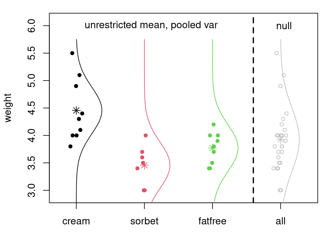

FIGURE 6.7: Illustrating ANOVA fit(s), overlaying Figure 6.6 with Gaussian fits under \(\mathcal{H}_0\).

Observe how fits with disparate means, to the left of the vertical dashed line, all have the same spread. This is because they use all \(s^2_{\mathrm{pool}}\). (The rightmost fit, under \(\mathcal{H}_0\), has wider spread via \(s^2\).) We know already, from our analysis earlier in §6.2, that the first two groups likely have the same variance. We could also test the other two pairs. I’ll spoil it for you: one rejects, and the other accepts. So it may be that a pooled variance model is not appropriate for these groups. This is a downside of the typical ANOVA setup. We’ve already seen, in §6.2, that the math is much easier with a pooled variance. The same is true here, too. We’ll look at relaxing this later, beginning with a homework exercise in §6.5.

The statistic preferred in an ANOVA doesn’t involve any assumptions about pooled variances; however, its distribution does. In fact, at first blush it would appear, rather, to involve separately estimated variances. Remember, the testing statistic is technically your choice. I’m showing you what’s canonical, which is usually based on a compromise between what works (what has good power, §A.2) and what has a distribution available in closed form. With MC, we’re less beholden to closed forms, but it’s important to make connections to established procedures.

Alright, here we go. Above, I said that the ANOVA test statistic relates the quality of unconstrained (\(\mu_j \ne \mu_k\)) fits under \(\mathcal{H}_1\) via \(\bar{y}_{\cdot j}\) to a constrained one (\(\mu \equiv \mu_1 = \mu_2 \dots = \mu_m\)) under \(\mathcal{H}_0\) via \(\bar{y}\). A neat identity that makes this possible is provided below.

\[\begin{align} \sum_{j=1}^m \sum_{j=1}^{n_j} (y_{ij} - \bar{y})^2 &= \sum_{j=1}^m \sum_{i=1}^{n_j} (\bar{y}_{\cdot j} - \bar{y})^2 + \sum_{j=1}^m \sum_{i=1}^{n_j} (y_{ij} - \bar{y}_{\cdot j})^2 \tag{6.9} \\ \mathrm{SST} &= \mathrm{SSR} + \mathrm{SSE} \notag \end{align}\]

Showing this is true is left as a homework exercise. You may have done one like this before in §3.5 #5. The second line above defines some acronyms for the components of the identity. \(\mathrm{SS}\) stands for “Sum of Squares”. The third letter – E, R or T – is supposed to help you remember which part is what, though I still get it confused.

• \(\mathrm{E}\) is for “Error”, which is a strange choice. All of these SSs are measuring (squared) errors of a sort; here it’s the error in predicting \(y_{ij}\) with \(\bar{y}_{\cdot j}\). Each component in the sum for \(\mathrm{SSE}\) is a scaled within-group variance estimate: \(\mathrm{SSE} = \sum_{j=1}^m (n_j - 1) s_j^2\). The more useful the grouping variable, the smaller the \(\mathrm{SSE}\).

sse <- sum((nj - 1)*s2j)

• \(\mathrm{R}\) is for “Regression”, which is awkward because we haven’t talked about what regression is yet. That comes in Chapter 7. Anyways, this one is measuring how different each within-group average \(\bar{y}_{\cdot j}\) is from the grand average \(\bar{y}\). The more useful the grouping variable, the larger the \(\mathrm{SSR}\).

ssr <- sum(nj*(ybarj - ybar)^2)

• \(\mathrm{T}\) is for “Total”. This one is easy to remember. \(\mathrm{SST} = (n-1) s^2\) under \(\mathcal{H}_0\), measuring quality of fit for all of the data around the grand average \(\bar{y}\).

sst <- ssr + sse

Well there you have it. Again, please don’t shoot the messenger. I bet the machine learning community (if it cared about ANOVA) would have come up with better shorthands. I’ll show you actual sse, ssr, and sst values from data later. They’re not germane to our discussion at this time.

Since the whole (\(\mathrm{SST}\)) equals the sum of its parts \((\mathrm{SSR}\) and \(\mathrm{SSE}\)), any of the parts over the whole is a proportion, and you can always get the third one from the other two. Compactly:

\[\begin{equation} 0 < r^2 \equiv \frac{\mathrm{SSR}}{\mathrm{SST}} = 1 - \frac{\mathrm{SSE}}{\mathrm{SST}} < 1. \tag{6.10} \end{equation}\]

Ratio \(r^2 = \mathrm{SSR}/\mathrm{SST}\), verbalized as “r-squared”, is also known as the coefficient of determination. The reason for the lettering \(r^2\) has to do with a correlation and linear regression connection coming later in Chapters 7 and 12. The reason for that strange name is that statisticians are bad at naming things. Quantity \(r^2\) is always positive because squares are positive.

r2 <- ssr/sst
r2

## [1] 0.5086

An \(r^2\) value may be interpreted in percent terms. The grouping, in this case by frozen treat type, explains 51% of the total variability in the data.

Quick digression on the inequalities in Eq. (6.10). These should technically not be strict – both should be \(\leq\) – but something is very wrong if you get an \(r^2\) that’s zero or one. You either have \(n_j = 1\) for some \(j\), or \(n_j > 1\) but with duplicated values, and/or \(m = n\). Those are degenerate cases with more estimated quantities than (unique) data values. You have a DoF problem, or a bug in your code.

Alright, back to ANOVA. The important thing to take away from all this is that a grouping is valuable, compared to not grouping at all (i.e., under \(\mathcal{H}_0\)), if it explains most of the variability. This is where the V in ANOVA comes from. If \(r^2\) is large, close to 1, then the grouping in question is valuable. As usual, “large” must be measured statistically, against its sampling distribution under \(\mathcal{H}_0\).

Conversely, if \(\mathrm{SSE}\) is small, then within-group averages \(\bar{y}_{\cdot j}\) are close to their \(y_{ij}\)-values, providing a good fit. The closer they are the smaller the aggregate squared distances, \(\mathrm{SSE}\), and therefore the larger amount left over in \(\mathrm{SSR}\). Coming full circle, \(\mathrm{SSR}\) is large when \(\bar{y}_{\cdot j}\) values are far from one another, and from the grand average \(\bar{y}\).

Summarizing: the grouping is useful when between-group variability, \(\mathrm{SSR}\), is large relative to within group variability, \(\mathrm{SSE}\). Turning that into a test involves inspecting those quantities under \(\mathcal{H}_0\), and forming a contradiction.

I suggest reading over the previous three paragraphs a few times to make sense of things. Refer back to Figure 6.7, Eq. (6.9) and subsequent bullets, and ponder. If you’re still struggling, don’t worry. I got it all wrong twice when writing those passages, because things were all twisted up in my head, before getting it right. Quantities like \(r^2\), and the three \(\mathrm{SS}\)s are just statistics.

It bears repeating that what matters is how a statistic looks under a sampling distribution implied by \(\mathcal{H}_0\). That’s actually pretty easy and comes next. The idea behind ANOVA is that if some \(\mu_j \ne \mu_k\), under the alternative hypothesis \(\mathcal{H}_1\), then these quantities will look “out-of-whack” relative to one another under the sampling distribution from \(\mathcal{H}_0\). Since they’re related to one another as a sum of parts (6.9), a ratio like \(r^2\) provides a nice, interpretable scalar statistic for inspection.

It turns out that a different, but related, ratio has some advantages mathematically. I’m going to quote it here, and talk more about it when it comes to closed-form calculations later. When testing via MC, we have more flexibility when it comes to the choice of test statistic.

\[\begin{equation} f = \frac{\mathrm{SSR}/(m-1)}{\mathrm{SSE}/(n-m)} \equiv \frac{\mathrm{MSR}}{\mathrm{MSE}} \tag{6.11} \end{equation}\]

msr <- ssr/(m - 1)
mse <- sse/(n - m)
f <-  msr/mse

You guessed it, the random \(F\) that you get by replacing \(y_{ij}\) with \(Y_{ij}\), etc., has an \(F\) distribution. But I’m getting ahead of myself. The \(\mathrm{M}\) in \(\mathrm{MSE}\) and \(\mathrm{MSR}\) stands for “Mean”, because we’re dividing by the number of DoF involved in the sums \(\mathrm{SSE}\) and \(\mathrm{SSR}\), respectfully. The reason for putting this here, as opposed to later when I get to the math version of the test, is so that I can draw a comparison between \(r^2\) and \(f\) values via MC.

ANOVA test by MC

That was complicated; I apologize. This is going to be a lot easier. Why? Because it’s like a two-sample (pooled variance) \(t\)-test from §5.2, but with \(m\) samples. And at the end we calculate \(R^2\) or \(F\), thinking now of them as random quantities. Finally, a comparison is drawn to observed versions: \(r^2\) or \(f\).

As with other examples involving a common mean \(\mu\) and/or variance \(\sigma^2\) under \(\mathcal{H}_0\), it doesn’t matter what values are used in the simulation. Your instinct may be to iterate over the \(m\) groups with a for loop, and there’s nothing wrong with that. However, a list representation makes things tidier with lapply and sapply and is more faithful to data structures for, and manipulation of, the observed data and its statistics. See comments below for how a for-loop variation might work instead.

N <- 1000000
mu <- sigma2 <- 1               ## any mu and sigma2 values work
R2s <- Fs <- rep(NA, N)         ## storage for both stats
for(i in 1:N) {

  ## draw under null hypothesis
  ## essentially a "for" loop {
  Ys <- lapply(nj, rnorm, mean=ybar, sd=sqrt(s2))

  ## within-group calculations
  Ybarjs <- sapply(Ys, mean)
  S2js <- sapply(Ys, var)
  ## } where the "for" loop would end
  
  ## grand average
  Ybars <- sum(nj*Ybarjs)/sum(nj)

  ## sums of squares
  SSEs <- sum((nj - 1)*S2js)
  SSRs <- sum(nj*(Ybarjs - Ybars)^2)

  ## sampled R^2 statistic
  SSTs <- SSEs + SSRs
  R2s[i] <- SSRs/SSTs

  ## sampled F statistic
  MSRs <- SSRs/(m - 1)
  MSEs <- SSEs/(n - m)

  ## f statistic
  Fs[i] <- MSRs/MSEs
}

Figure 6.8 provides views of both sampled statistics, \(R^2\) on the left and \(F\) on the right, with observed values overlayed as red vertical lines. ANOVA is always done as a one-tailed test. It could be done two-tailed, in the same way as other two-tailed tests (with a reflected statistic, etc.), but we’re not going to do it that way here so that everything will line up with library output, coming later. There’s also a good reason for doing things one-tailed, and I’ll get back to that later in §6.4 after I’ve covered some of the math.

par(mfrow=c(1, 2))
hist(R2s, main="")
abline(v=r2, col=2, lwd=2)
hist(Fs, main="")
abline(v=f, col=2, lwd=2)
legend("topright", "observed stat", lty=1, lwd=2, col=2,  bty="n")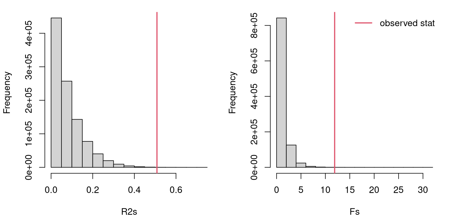

FIGURE 6.8: Histogram of sampled \(R^2\) (left) and \(F\)-values (right) for the scoop weight data under the null hypothesis, with observed statistics overlayed.

Looking at either of those histograms, it is clear that the observed statistic is extreme compared to its sampling distribution(s). This should be an easy reject of the null hypothesis, concluding that at least one pair of means differs. Code provided below calculates \(p\)-values in the usual way, under both stats/distributions.

pval.mc <- c(r2.mc=mean(R2s > r2), f.mc=mean(Fs > f))
pval.mc

##    r2.mc     f.mc 
## 0.000274 0.000274

In situations where both right tails are light, \(p\)-values under \(R^2\) or \(F\) are often the same or very close. \(R^2\) values are always between 0 and 1, and so its distribution doesn’t really have tails in quite the same way. This can impact how an \(r^2\) tail probability compares to an \(f\) one. However, in this particular instance, both distributions are “light” at their extremes, as shown in the figure. Both \(p\)-value calculations are also based on exactly the same pseudo-random numbers. So the two numbers are identical.

I prefer \(r^2\) because it’s both simpler, and has nice interpretation. Historically, \(f\) is preferred because of how the math turns out.

ANOVA test by math

Let’s begin by repurposing the analysis of §6.2 around Eqs. (6.2) and (6.3). That was really an adaptation of Eq. (3.16) from §3.2, where I introduced the \(t\)-test. Sorry about using all those equation references all at once. Bear with me. Referring back to Eq. (6.9) in the context of Chapter 3, we have

\[\begin{align} \mathrm{MSR} &= \frac{\mathrm{SSR}}{m-1} \sim \sigma^2 \chi^2_{m-1} & & \mbox{ and } & \mathrm{MSE} &= \frac{\mathrm{SSE}}{n-m} \sim \sigma^2 \chi^2_{n-m}. \tag{6.12} \end{align}\]

As in Chapter 3, I’ll wave my hands at this a little and offer the following justification that involves counting DoF in sums of squares. \(\mathrm{SST}\) involves estimating one quantity, \(\bar{y}\), and summing up \(n\) squares from \(y_{ij}\), and therefore has a \(\chi_{n-1}^2\) distribution. \(\mathrm{SSE}\) involves estimating \(m\) quantities and then summing up \(n\) squares. Since \(\mathrm{SST} = \mathrm{SSR} + \mathrm{SSE}\), we may deduce that \(\mathrm{SSR}\) involves \(n - m\) DoF. Compactly, \(n-1 = n-m + m - 1\).

A key feature of Eq. (6.12) is that \(\sigma^2\) is involved in the distribution of both \(\mathrm{MSR}\) and \(\mathrm{MSE}\). That way \(\sigma^2\) cancels out in the \(f\) ratio (6.11). This is where a pooled variance assumption (6.5) is pivotal. Without that, there’s no cancellation. In fact, it’s not clear at all what you’d get otherwise. An ordinary, unpooled two-sample \(t\)-test requires approximation, e.g., via the Welch test. Or, worse still, you fall deep into a rabbit hole and develop a whole new form of inference. (See discussion in §5.2.) That hole is \(m\)-fold deeper in an ANOVA context when you don’t pool variance across all \(m\) samples.

But when you do pool variance, everything falls out nicely. Combining Eqs. (6.3) and (6.4), the \(f\) statistic (6.11) – when viewed as a random variable for random \(Y_{ij}\), \(\bar{Y}_{\cdot j}\) and \(\bar{Y}\) – has the following distribution.

\[ F \sim F_{m-1, n-m} \]

A \(p\)-value for observed \(f\) under this distribution may be calculated by integrating into the right tail as follows.

pval.math <- pf(f, m-1, n-m, lower.tail=FALSE)
c(f.math=pval.math, pval.mc)

##    f.math     r2.mc      f.mc 
## 0.0002829 0.0002740 0.0002740

That’s pretty close to our MC variation. With data arranged into a data.frame, a library call could look like this.

fit <- aov(weight ~ type, data=ydf)
anova(fit)$Pr[1]

## [1] 0.0002829

That’ll take a little unpacking. The function aov fits the ANOVA model (6.5). If you want, you can inspect the intermediate fit object. I find that not very enlightening because of the way things are stored/presented. I’ll have to circle back to that later after I introduce multiple linear regression in Chapter 13, for which ANOVA is a special case.

The first argument to aov is a formula that explains how to interpret the second, data argument. Here, the formula explains that weight is \(y\) and type is the grouping. In this context, type is sometimes called an explanatory or independent variable, and weight is the dependent or response variable, or outcome. More on these vocabulary words is provided near Table 7.1 in Chapter 7.

Calling anova on the fit provides the actual analysis. I’ve extracted the \(p\)-value, above, for quick comparison to the other calculations. The full output is possibly of interest, so it’s provided below.

anova(fit)

## Analysis of Variance Table
## 
## Response: weight
##           Df Sum Sq Mean Sq F value  Pr(>F)    
## type       2   4.31   2.153    11.9 0.00028 ***
## Residuals 23   4.16   0.181                    
## ---
## Signif. codes:  0 '***' 0.001 '**' 0.01 '*' 0.05 '.' 0.1 ' ' 1

This is what is known as an “ANOVA table”, summarizing the outcome of intermediate steps via key quantities. We have all of the ingredients from our own calculations, and can thus hand-build our own ANOVA table as follows. See Table 6.1.

tab <- cbind(c(m - 1, n - m), c(ssr, sse), c(msr, mse), 
  c(f, NA), c(pval.math, NA))
tab <- rbind(tab, c(sum(tab[,1]), sum(tab[,2]), rep(NA, 3)))
rownames(tab) <- c("Regress", "Error", "Total")
colnames(tab) <- c("DoF", "SS", "MS", "fstat", "pval")
kable(round(tab, 5), caption="ANOVA table for scooping weights.")

TABLE 6.1: TABLE 6.2: ANOVA table for scooping weights.

	DoF	SS	MS	fstat	pval
Regress	2	4.306	2.1529	11.9	3e-04
Error	23	4.160	0.1809
Total	25	8.466

Notice I’ve renamed things a little bit. The biggest change is in the row labels. The “E” in \(\mathrm{SSE}\) is for “Error”, but R calls this “Residuals” which starts with an R, clashing with \(\mathrm{SSR}\) and potentially causing confusion. So I use “Regress” and “Error”. That way things line up better with notation introduced earlier, which is fairly standard. I’ve also added an extra “Total” row. This doesn’t appear in the R output, but is also typical for ANOVA tables and is relatively self-explanatory in light of Eq. (6.5).

ANOVA tables were helpful back in the day to check your bookwork, especially in a classroom, homework, or exam context where you’re doing a lot of it by hand. It’s so easy to make a little mistake and throw everything off. Neatly arranging intermediate output allows you, or a grader, to trace back through your calculations to see where the problem might be. (Always show your work!) ANOVA tables are less useful in a modern context, although perhaps you could still be asked to fill one out on an exam.

Just in case you encounter it – I’ve got a good one for you in §6.5 – it’s important to know how the rows and columns work together. Observe that the third column is the ratio of the first two, and the fourth one is the ratio of the two entries of the previous one. (I’ve deliberately been a little terse in that explanation as a nudge to you to investigate what, exactly, I might mean.)

6.4 Multiple testing hazard

I’ve said there’s a connection between ANOVA and a two-sample, pooled-variance \(t\)-test. When \(m=2\), the models (6.5) are identical. They use different test statistics (\(f\) and \(t\), respectively), which are measured against different sampling distributions. Are they different tests? Let’s find out.

But wait, watch me kill two birds with one stone while pivoting to a new topic. We’ve determined, with the ANOVA analysis above, that at least one of these three things is not like another. One way to get to the bottom of that is to explore groups pairwise. R code below loops over all pairs, first performing \(t\)-tests, then performing \(m=2\) ANOVA tests on pairs. These are stored in opposing triangles of a symmetric matrix for easy viewing, provided Table 6.3.

## matrix storing p-values for all pairs
pval.pairs <- matrix(NA, nrow=m, ncol=m)
colnames(pval.pairs) <- rownames(pval.pairs) <- names(ylist)

## loop over all pairs 
for(i in 1:(length(ylist) - 1)) {
  for(j in (i + 1):length(ylist)) {

    ## pooled-variance t-test
    pval.pairs[i,j] <- t.test(ylist[[i]], ylist[[j]], var.equal=TRUE)$p.val

    ## anova test
    r <- ydf$type %in% c(i,j)
    pval.pairs[j,i] <- anova(aov(weight ~ type, data=ydf[r,]))$Pr[1]
  }
}

## pretty table
kable(pval.pairs, 
  caption="$p$-values from ANOVA (rows) and 
  pooled-var $t$-tests (columns).")

TABLE 6.3: TABLE 6.4: \(p\)-values from ANOVA (rows) and pooled-var \(t\)-tests (columns).

	cream	sorbet	fatfree
cream		0.0014	0.0038
sorbet	0.0014		0.0598
fatfree	0.0038	0.0598

Two key takeaways from the table are as follows:

1. The \(p\)-values in the \((i,j)^{\mathrm{th}}\) cell match those in the \((j,i)^{\mathrm{th}}\) one, so the tests have the same outcome. Ask the same question, get the same answer. That’s a relief. This explains, at least in part, why ANOVA is a one-tailed test, because that’s how you match the result of a two-tailed, pooled variance \(t\)-test. In a way, ANOVA is already two-tailed since it looks at squared deviations from averages. Squares treat under- and over-prediction symmetrically.

2. Regular, full-fat ice-cream seems to be heavier than both sorbet and fat-free ice cream. But there’s no detectable weight difference between sorbet and fat-free ice cream.

You might be wondering about what the value of ANOVA is, when you can just do a bunch of paired \(t\)-tests. The answer is hidden in the name of this section. Simply put, the more questions you ask, the more chances you have of messing it up. If what you want to know is whether (at least) one thing is not like another, you’re more likely to get it wrong if you ask \({m \choose 2} = m(m-1)/2\) questions, which is 3 when \(m=2\), than if you just ask one question.

Our hypothesis tests are set up to reject \(\mathcal{H}_0\) when the \(p\)-value is below \(\alpha = 0.05 = 1/20\). So \(1/20\) is our chance incorrectly rejecting the null hypotheses (a so-called Type-I error), when there’s a close call (\(p\) near \(\alpha\)). Those chances compound each time we look at a \(p\)-value and compare it to \(\alpha\). When \(m \geq 7\) we have \(m(m-1)/2 > 20\), possibly much bigger than 20. So if you proceed pairwise, with 20+ paired tests, you’re essentially guaranteed to get something wrong. It’s much safer, though not easier, to do an \(m\)-fold ANOVA, which asks just one question. If and when you reject the \(m\)-fold ANOVA null, you might find it handy to drill down with smaller tests.

I’m describing what’s known as the multiple testing problem, but I prefer the word hazard over problem. There are some good ways to work around the hazard, and I encourage you to read more. There are many contexts where you might be looking for a needle in a haystack, and thus feel compelled to do thousands of tests. Great examples come from genomics and genetic association studies where comparisons (mini-experiments) are drawn on tens of thousands of genes. That isn’t going to work out well without some adjustment.

Ignoring the multiple testing hazard is a common mistake known as \(p\)-hacking or data dredging. “Hacking” shouldn’t have a negative connotation. There are plenty of noble hackers. Nonetheless, you don’t want to be caught \(p\)-hacking. Instead, remember to make a Bonferroni correction, or make some other similar adjustment, to account for compounding Type-I error.

6.5 Homework exercises

These exercises help gain experience with one- and two-sample variance tests, and ANOVA. When the question involves performing a test for data, I suggest doing it both ways: via MC and with math. Check with your instructor for details.

Do these problems with your own code, or code from this book. I encourage you to check your work with library functions like var.test and anova. Check with your instructor first to see what’s allowed. Unless stated explicitly otherwise, avoid use of libraries in your solutions.

#1: MC CI for one sample

Write code that calculates a CI for \(\sigma^2\) in a Gaussian sample via MC (6.1). Use your code to calculate the interval for ice cream scoops in §6.1, and compare your result to values stored in CI.math.

#2: monty.var for one- and two-samples

Write a function called monty.var that automates testing and CI calculation (see #1 above) for one- and two-sample variance tests. Follow specifications similar to monty.bern and monty.t one- and two-sample tests from earlier chapters, including optional visuals. I don’t need to rehash all that here. Just make sure you cover both MC and math-based procedures.

Hint: many of the following questions are easier after this one is squared away.

#3: Postal scales

A budget supplier of postage scales claims that its scales are accurate for letters weighing less than 10 oz because the standard deviation of measurements, across weights and scales, is 0.1 oz (i.e., \(\sigma^2 = 0.01\)). Twenty-five scales were tested with a single letter weighing 2 oz and the sample variance was \(s^2 = 0.02\). Do you have enough evidence to refute the supplier’s claim?

#4: Pitching machine

A pitching machine, used by baseball players to practice hitting, is designed to serve up baseballs at a desired speed, e.g., 80 mph, with a standard deviation of 1 mph. Radar, accurate to 1/100 mph, was used to measure the speeds of ten pitches with the machine set to 80 mph.

mph <- c(80.05, 79.82, 80.13, 80.18, 79.81, 79.1, 80.03, 80.41, 
  80.30, 79.71)

What do you think about the actual variance of balls flung by this pitching machine?

#5: Nitrogen absorption from fertilizer

Two kinds of fertilizer (A and B) are tested in a laboratory, where an experiment was performed to measure the nitrogen absorption rate for a corn crop. Seven plots of corn with fertilizer A yielded a sample absorption rate with \(s_A^2 = 2.1\) (in units of %-squared). Nine plots of corn with fertilizer B yielded \(s_B^2 = 0.8\). Is the variability of nitrogen absorption similar for the two fertilizers?

#6: Homemade energy drinks

A budget- and health-conscious triathlete has been experimenting with a new energy drink recipe that contains 1 liter of water, 80 grams of sugar, 2 ml of salt, and 5 tablespoons of lime juice. She has two methods of combining these ingredients. Method A involves following the recipe on a per-bottle basis, filling one at a time in this way. (Note: 1 liter bottles are used, so the recipe includes slightly less water than is prescribed, so all the other ingredients can fit.) Method B involves combining all the ingredients (approximately 18-fold) into a five-gallon jug, mixing, and the dispensing into 18 one-liter bottles. She wants to know if there is any difference in the variance of sugar content, measured in g/L, between the two methods. Some measurements are provided below.

A <- c(85.1, 85.0, 85.1, 84.8, 85.1, 84.8, 83.5, 84.9, 84.2, 85.0)
B <- c(76.3, 75.8, 77.2, 75.7, 76.7, 74.9, 75.1, 79.8, 76.9, 75.4, 
  75.3, 75.5, 75.3, 75.8, 75.7, 75.8, 75.7, 78.1)

What do you think?

Follow-on challenge question: there is one data point in the B set which, if you remove it from the data set the outcome of the test changes at the 5% level. Which one do you think it is and why? (Confirm your intuition.)

#7: Return on investment

Refer back to roi$company and roi$industry from §2.5, via roi.RData on the book webpage.

load("roi.RData")

Does there seem to be any difference in ROI variance between companies that use the IT product in question and the industry at large?

#8: ANOVA SS identity

Show the sum-of-squares (SS) identity quoted in Eq. (6.9). See the hint provided for §3.5 #5. Be careful, in general \((a + b)^2 \ne a^2 + b^2\). As always when “showing” an equality: start on the left-hand side, and manipulate the expression with one (equal) modification at a time, ending eventually with the expression on the right-hand side.

#9: monty.ANOVA

Write a function called monty.ANOVA that automates ANOVA testing by MC and using closed-form, mathematical calculations, including optional visuals. You know the drill by now. Assume a list representation, like ylist above in §6.3. In addition to explicitly proving a $pval entry in your output list containing the \(p\)-value, provide $tab output that contains ANOVA table information like in Table 6.1.

Hint: many of the following questions are easier after this one is squared away.

#10: Partial ANOVA table

The ANOVA summarized in Table 6.5 is only partially completed. Complete the table and use it to answer the following prompts.

TABLE 6.5: TABLE 6.6: Partial ANOVA table.

	DoF	SS	MS	fstat	pval
Regress	4
Error		964
Total	53	1123

• How many groups were in the study?
• How many total observations were in the study?
• What is the outcome of the hypothesis test?

This is a classic exam-type question because you don’t need to do any serious coding, just arithmetic and a pf calculation.

#11: Puppy chow

A study was performed in partnership with a dog breeder to compare five different premium dog food brands. Weened, but otherwise “newborn” puppies were fed fixed servings of a single brand of dog food for six months. Their weights were recorded at the beginning and end of the study, and that difference (their weight gain in pounds) was recorded. Those values are provided below.

wtgain <- list(
  A=c(44, 49, 50, 50, 49),
  B=c(51, 52, 52, 52, 50, 49),
  C=c(55, 52, 53, 54, 53, 50, 51),
  D=c(51, 50, 52, 49, 51),
  E=c(51, 54, 56, 53, 55, 56))

Is there any difference between these dog foods as regards weight gain?

#12: Fisher’s iris

Possibly the most famous ANOVA-style data set is Fisher’s iris data, available in R as a built-in data.frame called iris. These data were collected by Anderson (1935), and Fisher’s analysis was published a year later in a – now highly controversial outlet – on eugenics (Fisher 1936). A similar data set was included in the S language, a precursor to R (Becker, Chambers, and Wilks 1988). A quick peak at some of the columns are provided below.

summary(iris[,2:5])

##   Sepal.Width    Petal.Length   Petal.Width        Species  
##  Min.   :2.00   Min.   :1.00   Min.   :0.1   setosa    :50  
##  1st Qu.:2.80   1st Qu.:1.60   1st Qu.:0.3   versicolor:50  
##  Median :3.00   Median :4.35   Median :1.3   virginica :50  
##  Mean   :3.06   Mean   :3.76   Mean   :1.2                  
##  3rd Qu.:3.30   3rd Qu.:5.10   3rd Qu.:1.8                  
##  Max.   :4.40   Max.   :6.90   Max.   :2.5

The grouping variable is iris Species: Setosa, Versicolor, and Virginica. These comprise just three of 300+ species of iris. There are four measured responses available for analysis, and which might vary by species. Those are sepal length and width, and petal length and width. I cut sepal width (iris[,1]) out of the summary above to save space. Don’t exclude it from your analysis.

What do you think? Do iris sepal and petal measurements vary by species? Hint: one convenient way to turn two vectors, one with real-valued measurements and another factor grouping variable, into a list is with split in R.

#13: Warm-blooded T-rex?

Data supporting this question come from the Sleuth3 library (Ramsey et al. 2024), which you will need to install. See ex0523.

library(Sleuth3)    ## first do install.packages("Sleuth3")
summary(ex0523)

##      Oxygen          Bone   
##  Min.   :10.6   Bone10 : 6  
##  1st Qu.:11.3   Bone11 : 5  
##  Median :11.5   Bone12 : 5  
##  Mean   :11.6   Bone4  : 5  
##  3rd Qu.:11.9   Bone5  : 5  
##  Max.   :12.4   Bone7  : 5  
##                 (Other):21

(See split hint above in #12.)

These quantities, originally from Barrick and Showers (1994) and repurposed for a popular textbook (Ramsey and Schafer 2013), consist of several measurements of the oxygen isotopic composition of bone phosphate, which is related to body temperature at formation, in each of twelve bone specimens from a single Tyrannosaurus Rex skeleton. Differences in means at different bone sites would indicate non-constant temperatures throughout the body. This would be expected in warm-blooded animals, but not cold-blooded ones. Do these data comprise evidence that T-rex was warm blooded?

#14: Non-pooled ANOVA variance

This one is a challenge problem, but totally doable. Also, I can think of a lot of different ways to do it, so have fun!

How would you modify a MC-based ANOVA test in order to accommodate a non-pooled variance setup? That is, the model is as follows

\[ Y_{ij} \stackrel{\mathrm{iid}}{\sim} \mathcal{N}(\mu_j, \sigma_j^2) \quad\quad i=1,\dots,n_j \ \mbox{ and } \ j=1,\dots,m, \]

but everything else, including hypotheses (6.6), is just as in §6.3.

You might draw inspiration from two-sample \(t\)-tests (with unpooled variance) from §5.2. Aim for a hybrid between that setup and ordinary ANOVA.

Go back through the earlier ANOVA data sets from §6.3 and exercises #11–13 above. How does relaxing a pooled variance assumption change, or not, the outcome of the tests?

References

Anderson, E. 1935. “The Irises of the Gaspe Peninsula.” Bulletin of the American Iris Society 59: 2–5.

Barrick, R. E., and W. J. Showers. 1994. “Thermophysiology of Tyrannosaurus Rex; Evidence from Oxygen Isotopes.” Science 265: 222–24.

Becker, R. A., J. M. Chambers, and A. R. Wilks. 1988. The New S Language. Wadsworth & Brooks/Cole.

Fisher, R. A. 1936. “The Use of Multiple Measurements in Taxonomic Problems.” Annals of Eugenics 7 (Part II): 179–88.

Millard, S. P. 2013. EnvStats: An r Package for Environmental Statistics. New York: Springer. https://www.springer.com.

Ramsey, F. L., and D. W. Schafer. 2013. The Statistical Sleuth: A Course in Methods of Data Analysis, 3rd Edition. Brooks/Cole Cengage Learning.

Ramsey, F. L., D. W. Schafer, J. Sifneos, B. A. Turlach, N. Horton, L. Loi, K. Aloisio, R. Zhang, and R. Pruim. 2024. Sleuth3: Data Sets from Ramsey and Schafer’s “Statistical Sleuth (3rd Ed)”. https://CRAN.R-project.org/package=Sleuth3.