Chapter 3 A little math: inference

There’s not too much math in this book, I promise. Like 99% of it is in Chapters 3-4. Mostly my goal in this book is to show you how much of statistics can be math-free with a computer. Yet, a lot of statistical fundamentals are rooted in math, and I want to show you how people usually do things. So we’ve gotta do this. I’ll try to make it as painless as possible.

At times I’ll use the words analytic or closed form to describe the methods in this chapter. Sometimes both at the same time (analytic closed form). This is just me being fancy with big words. By either or both, I simply mean “using math”, as opposed to numerical methods like Monte Carlo (MC). My use of “analytic” in this context is highly colloquial, and wouldn’t align well with the technical definition at that Wikipedia link. “Closed form” is appropriate, since it basically means “you get a function, expression or number”, as opposed to “you get samples” (MC) or “you iterate until convergence” (other numerical procedures). Asymptotic methods, like those in Chapter 4, also provide closed forms, but those are approximate. The ones in this chapter are exact.

Almost everything here is an application of something you know already from high school math and probability. That is, assuming you took calculus in high school. I didn’t, believe it or not. I wasn’t the best high school student; I thought I was an athlete not a scholar. Hoping to satisfy a “gen-ed” requirement with as little hassle as possible, I re-took pre-calculus in my third quarter at UC Santa Cruz (UCSC). I was surprised to like it. I give the credit to an excellent professor. I didn’t take the calculus sequence at UCSC until my second year. Wouldn’t you know it, I ended up a math major, and eventually a college professor.

Anyways, most of the stuff in this chapter is pretty straightforward conceptually, but let me warn you that getting good at it will take practice. You have to practice this stuff, like anything else in math (or life), to feel comfortable with it. There will be a few things that I’ll waive my hands at because the math is hard, but the result is too important to omit. That importance is either conceptual, in the sense that it reveals a beautiful truth about how numbers and randomness work. Or it’s a linchpin, in the sense that we can’t move on without it, but otherwise it’s pretty trivial and not very interesting. There’s like one or two of each of those coming up here and in Chapter 4.

My goal is two-fold: (1) to give you a cookbook/recipe framework for the rest of the book; (2) to circle back to the coin-flipping and location examples of Chapters 1–2, showing how binom.test and z.test library functions really work. Then we’ll talk about \(t\)-tests, the most famous of all tests, and about confidence intervals.

3.1 Maximum likelihood

It helps to have an “automatic” procedure for estimating unknown quantities, like parameters in probabilistic models. Think \(\theta\) for Bernoulli data in Chapter 1 or \(\mu\) and \(\sigma^2\) for Gaussian data in Chapter 2. Here, I’ll generically use \(\theta\) as the unknown parameter. This quantity may be a scalar, like in the Bernoulli case, or it may be a \(p\)-vector, like in the Gaussian case where \(\theta = (\mu, \sigma^2)\) and \(p=2\).⁵ In the next little bit, it’s fine to think of \(\theta\) as a single, unknown number. What’s that? Did someone say Hessian? No? Oh, never mind.

Let \(f(y; \theta)\) denote the probability mass or density function for random variable \(Y\), as determined by parameter \(\theta\). That’s for a single \(y\). Usually we have a data set of \(n\) observations, notated as \(y_1,\dots,y_n\), modeled as all having the same distribution (the same probability mass or density function), independent of one another conditional on a common setting for the parameter \(\theta\). The short hand for that is iid. So far, I’m just rehashing §1.2. Hold tight.

Recall that a joint density or mass factorizes as a product (1.2) under an iid assumption. I’ll rewrite things here to be more generic with \(f\) as a density or mass, whereas Eq. (1.2) favors a discrete random variable via \(\mathbb{P}(Y_i = y_i)\). This product is known as the likelihood

\[ L(\theta) \equiv L(\theta; y_1, \dots, y_n) = f(y_1, \dots, y_n; \theta) = \prod_{i=1}^n f(y_i ; \theta). \]

So the likelihood is the joint mass or density, and it’s a product of individual densities when observations are iid. Why have a special name for it? One reason is to elevate its importance. Another reason is because of how we are meant to think about it in the context of parameter \(\theta\). A density or mass \(f\) is saying something about \(Y\) or \(Y_i\) for particular \(\theta\). With \(f\) we think of \(y\) or \(Y\) as varying given fixed \(\theta\). For \(L\) we think of varying \(\theta\) for fixed \(y_1,\dots, y_n\). A lot of times we abbreviate with \(L(\theta) \equiv L(\theta; y_1, \dots, y_n)\) to emphasize focus on \(\theta\), not \(y\).

For different values of \(\theta\), the quantity \(L(\theta)\) may be larger or smaller depending on how probable observed \(y_1, \dots, y_n\) values are. It makes sense to target the value of \(\theta\) that, under the model \(f\), makes the observed data most probable.

\[\begin{equation} \hat{\theta} = \mathrm{argmax}_\theta \; L(\theta) \tag{3.1} \end{equation}\]

This is called maximum likelihood estimation (MLE), and \(\hat{\theta}\) is the maximimum likelihood estimate. The E in MLE is interchangeably estimation, estimate and estimator (more on that later). It’s common to put hats on estimates of parameters in statistics, whereas un-hatted ones are stand-ins for other values like the “true”, unknown value generating the data. The \(\mathrm{argmax}\) is just a fancy way of saying “the argument (\(\theta\)) that maximizes”.

In the case of a Bernoulli distribution, we saw in Eq. (1.3) that \(L(\theta) = \theta^{\sum y_i} (1- \theta)^{n - \sum y_i}\). Recall that \(\sum y_i\) is short for \(\sum_{i=1}^n y_i\). I mentioned how this sum is all you need to characterize the joint distribution, or in this case to evaluate (or maximize) the likelihood. It is said that \(\sum_i y_i\) is a sufficient statistic, or sometimes we say “sufficient for \(\theta\)”, because it’s all you need from the data to decide on \(\theta\) through the likelihood. You just need the number of heads, or equivalently the number of tails (and \(n\)).

How to do that? How to solve for \(\hat{\theta}\) in Eq. (3.1)? The answer is derivatives. Optimization is one of the most important applications of differential calculus. The basic program is this. Take the derivative of the function you wish to optimize with respect to the variable you want to dial in, set equal to zero and solve. (And don’t forget to check that the critical point you’ve found is actually a minimum.)

When maximizing likelihoods, there’s actually one more, or rather one preliminary, step that’s required. It can be difficult to take the derivative of \(L(\theta)\), like in Eq. (1.3), in its raw form because it’s a product of exponentiated terms. That means messy applications of product and power rules for differentiation. It’s even harder – can even be impossible – to solve after setting to zero. Instead, practitioners take the logarithm of the likelihood, working with \(\ell(\theta) = \log L(\theta)\) before taking derivatives. The log-likelihood is also known as the score. This doesn’t really change the answer since

\[ \mathrm{argmax}_\theta \; \ell(\theta) = \mathrm{argmax}_\theta \; L(\theta) \quad \mbox{ where } \quad \ell(\theta) \equiv \log L(\theta) \]

because \(\log\) is a monotonic transformation, which preserves the locations of critical points.

Note that I’m generically writing \(\log\), since it doesn’t matter what base. Any of \(\log_{10}\), \(\log_2\) or \(\ln \equiv \log_e\) would be fine. You can change bases by multiplying by a constant, and that doesn’t change the location of critical points. In statistics, when someone writes \(\log\) without a base, they mean natural log (\(\ln \equiv \log_e\)), unless otherwise clarified, because many densities involve the inverse of \(\ln\) which is \(\exp\). We’ll come back to that in just a minute.

Logarithms have many nice properties. They’re both beautiful and intimidating. The main thing they do for us, in the context of maximizing likelihoods, is turn products into sums. They also bring powers down as multiples, which is really the same thing. Sums are easier to work with than products when it comes to derivatives; same for powers/multiples. Both make solving for critical points easier as well. Let me show you.

Toss up MLE

Consider a log Bernoulli (1.3) likelihood, and derivative-based maximization for the MLE.

\[\begin{align} \mbox{log-likelihood} && \ell(\theta) &= \left(\sum_{i=1}^n y_i \right) \log \theta + \left(n - \sum_{i=1}^n y_i \right) \log(1 - \theta) \notag \\ \mbox{derivative} && \ell'(\theta) &= \frac{\sum_{i=1}^n y_i}{\theta} - \frac{n - \sum_{i=1}^n y_i}{1 - \theta} \tag{3.2} \\ \mbox{solve} && 0 & \stackrel{\mathrm{set}}{=} \frac{\sum_{i=1}^n y_i}{\hat{\theta}} - \frac{n - \sum_{i=1}^n y_i}{1 - \hat{\theta}} = \sum_{i=1}^n y_i - n \hat{\theta} \notag \\ && \hat{\theta} &= \frac{1}{n}\sum_{i=1}^n y_i \equiv \bar{y} \notag \end{align}\]

What a cool result! The rate of heads, i.e., the average of the 0s and 1s representing the \(n\) coin flips, is the value of \(\theta\) that makes the observed \(y_1, \dots, y_n\) most probable.

Recall that the statistic we chose, a sum of binarized flips (or count of heads), is the same as \(s_n = n\hat{\theta}\). I used this \(s_n\) as a statistic in a hippopotamus test (1.4) for \(\theta\). In the code below, I’m using s and n variables defined in Chapter 1 for our coin-flipping data.

that <- s/n     ## s and n defined in Chapter 1
that

## [1] 0.6

So not only does an MLE give us an automatic way to estimate a parameter, with a nice (most probable) interpretation, but it gives us an automatic statistic for testing as well. I could have taken \(s_n = \hat{\theta}\), i.e., dividing the count by \(n\), but that wouldn’t have changed things much beyond scaling labels on the \(x\)-axis in Figure 1.1. Table that thought for the moment so I can present another example first, and then we’ll come back to it.

Location MLE

Now take a look at the Gaussian location model (2.1) from Chapter 2. I talked about some of the properties of the intuitive estimator \(\hat{\mu} = \bar{y}\), like unbiasedness and efficiency. I never actually wrote down the joint distribution for all \(y_1, \dots, y_n\). This is a good thing, because it allows me to work here from scratch and show you everything from start to finish.

Recall that the model is \(Y_i \stackrel{\mathrm{iid}}{\sim} \mathcal{N}(\mu, \sigma^2)\), for \(i=1,\dots, n\). So we have:

\[\begin{align} & \mbox{1: joint via iid} & f(y_{1:n}; \mu, \sigma^2) &= \prod_{i=1}^n \frac{1}{\sqrt{2 \pi \sigma^2}} \exp \left\{ -\frac{(y_i - \mu)^2}{2\sigma^2} \right\} \notag \\ & \mbox{2: re-label and distribute} & L(\mu, \sigma^2) &= \left( 2 \pi \sigma^2 \right)^{-n/2} \exp\left\{- \frac{1}{2\sigma^2} \sum_{i=1}^n (y_i - \mu)^2 \right\} \notag \\ & \mbox{3: log and simplify} & \ell(\mu, \sigma^2) &= c - \frac{n}{2} \log \sigma^2 - \frac{1}{2\sigma^2} \sum_{i=1}^n (y_i - \mu)^2 \notag \\ & \mbox{4: differentiate} & \frac{\partial\ell}{\partial \mu} &= - \frac{2}{2\sigma ^2} \sum_{i=1}^n (y_i - \mu)(-1) \tag{3.3} \\ & \mbox{5: set to 0 and simplify} & 0 &\stackrel{\mathrm{set}}{=} - n \hat{\mu} + \sum_{i=1}^n y_i \notag \\ & \mbox{6: solve} & \hat{\mu} &= \frac{1}{n} \sum_{i=1}^n y_i \equiv \bar{y}. \notag \end{align}\]

Would you look at that! The MLE is, again, the simple, intuitive estimate. Is that going to happen every time? No. I’ll show you in just a moment. First, a little commentary.

When I say “distribute”, like in Step 2, I mean push the product into the exponent, where it becomes a sum. This isn’t strictly necessary, but I think it looks a little neater. When you take the log in Step 3, you can do it on the product (which will become a sum) without hassle. You’ll have a little more work to simplify things. And when I say “simplify”, this relies on your algebra skills and could sometimes be laborious, often depending on how you set things up earlier. The constant in Step 3 is really \(c = - \frac{n}{2} \log 2 \pi\). Since this doesn’t depend on any of the parameters, \(\mu\) or \(\sigma^2\), it’s not really relevant. When taking a derivative, like in Step 4, these terms evaluate to 0. Don’t forget your chain rule! Finally, you may not always be able to do Step 6, the solving part. It’s not about you. I shall limit our focus in this book to situations where this is possible.

Just to have it coded up for stuff coming later, here is the \(\hat{\mu}\)-value using data from the heights analysis of Chapter 2. This is the same value as what I was calling s earlier. Our MLE and test statistic for “location” are the same, which happens a lot. In the code below, I’m using y defined in Chapter 2 from our heights analysis.

muhat = mean(y)   # y defined in Chapter 2, where s = muhat
muhat

## [1] 66.62

That was just for one of the two parameters, \(\mu\). What about \(\sigma^2\)? We have everything we need up to Step 3. Things change from Step 4 because we must now differentiate with respect to \(\sigma^2\) instead.⁶

\[\begin{align} & \mbox{4: differentiate} \quad\quad & \frac{\partial\ell}{\partial \sigma^2} &= - \frac{n}{2\sigma^2} - \frac{1}{2(\sigma^2)^2} \sum_{i=1}^n (y_i - \mu)^2 \tag{3.4} \\ & \mbox{5: set to 0 and simplify} \quad\quad & 0 &\stackrel{\mathrm{set}}{=} -n + \frac{1}{\sigma^2} \sum_{i=1}^n (y_i - \mu)^2 \notag \\ & \mbox{6: solve} \quad\quad & \hat{\sigma}^2 &= \frac{1}{n} \sum_{i=1}^n (y_i - \mu)^2 \notag \end{align}\]

These two derivatives – technically partial derivatives – form a gradient \(\nabla \ell\). Setting the gradient to zero and simultaneously solving for the MLE of all/both parameters at once is the same as doing them one at a time, when possible, if we also plug in the ones we’ve found along the way. In other words, plug in \(\hat{\mu}\) when solving for \(\hat{\sigma}^2\). So the MLE for \(\sigma^2\) in a Gaussian model is

\[\begin{equation} \hat{\sigma}^2 = \frac{1}{n} \sum_{i=1}^n (y_i - \bar{y})^2. \tag{3.5} \end{equation}\]

Quick digression: it turns out that this estimator is biased because \(\mathbb{E}\{\hat{\sigma}^2\} = \frac{n-1}{n} \sigma^2\). You’re asked to show this as an exercise in §3.5. However, it’s asymptotically unbiased since \((n-1)/n \rightarrow 1\) as \(n \rightarrow \infty\). We’ll talk a lot more about asymptotics in Chapter 4. This “bias” is why statisticians prefer another estimate

\[\begin{equation} s^2 = \frac{1}{n-1} \sum_{i=1}^n (y_i - \bar{y})^2, \tag{3.6} \end{equation}\]

because this one is unbiased. Here is what we would calculate with our heights data from Chapter 2.

s2 <- var(y)
c(s2, sigma2)

## [1] 4.592 6.250

R automatically divides by \(n-1\) when estimating a variance. This is a common choice because of the bias correction, giving up some optimality for good average-case behavior. Notice that this s2 value is different than the sigma2 one used in Chapter 2. More on this in §3.2.

Another reason Eq. (3.6) is preferred over the MLE is because it makes sense when \(n=1\). Notice that you’ll get 0 from the sum in this case because \(\bar{y} = y_1\) and \(n-1\) evaluates to zero for \(n=1\). So that’s a \(0/0\) fraction which is undefined. If you use \(\hat{\sigma}^2\) instead, you get \(0/1 = 0\) which is just wrong. You can’t have zero variance – the smallest possible variance – from just one observation. Nonsense! Better for variance to be undefined when \(n=1\). You need to see more than one different thing to detect how they can vary.

Alright, back to MLEs. Maximizing the likelihood gives you an automatic, procedural way to solve for “good” estimates of parameters to your model. You get the best fitting parameters to your data in a certain sense. This is so important, that I’m going to wrap it into Alg. 3.1. Therein I use a generic parameter \(\theta\) and density or mass \(f(y ; \theta)\). The parameter \(\theta\) may be scalar, as in a Bernoulli experiment, or it may be vectorized, e.g., in a Gaussian/location experiment where \(\theta = (\mu, \sigma^2)\). When derivatives are taken, I use gradient/partial derivative terminology even if \(\theta\) is scalar. If I do a good job here, you should be able to follow this procedure in any (iid) inferential setting.

Algorithm 3.1: Maximum Likelihood Estimation

Assume you have iid data \(y_1,\dots, y_n\), under a statistical model described by density or mass function \(f(y; \theta)\) for some parameter \(\theta\) with \(p\) components.

Then

1. Characterize the joint density/mass as a product where “[write it out]” stands for using the mathematical expression for the density or mass within the product.

\[ f(y_1, \dots, y_n; \theta) = \prod_{i=1}^n f(y_i; \theta) = \mbox{[write it out]} \]

2. Relabel as likelihood \(L(\theta)\), distribute the product through so it becomes a sum (when possible) and simplify as much as you can.

\[ L(\theta) = \mbox{[what you wrote out, but simplified with $\sum$ instead of $\prod$]} \]

3. Take a logarithm and simplify even further. Look for constants \(c\) representing (possibly complex) additive terms that are not a function of \(\theta\).

\[ \ell(\theta) = \log L(\theta) \quad \quad \mbox{where $\log$ means $\ln = \log_e$} \]

4. Take the gradient with respect to \(\theta\), formed of partial derivatives over its components \(\theta = (\theta_1, \dots, \theta_p)\).

\[ \nabla \ell = \left(\frac{\partial\ell}{\partial \theta_1}, \dots, \frac{\partial\ell}{\partial \theta_p}\right) \]

5. Establish the likelihood equations by setting that gradient to zero and simplifying.

\[ 0 \stackrel{\mathrm{set}}{=} \nabla \ell \Big{|}_{\theta = \hat{\theta}} \]

6. Solve those likelihood equations, which you can do one of two ways.

• One at a time for each \(\theta_j\), for \(j=1,\dots, p\), in any order.
• Or simultaneously for all components of \(\hat{\theta}\) at once.

Return \(\hat{\theta}\).

Some notes on a couple of those steps. If you did Step 3 right, taking the \(\log\), then you shouldn’t have any exponential (\(\exp\)) or powers left in your expression. Now on to Step 6. In our Gaussian example, we solved for each parameter one at a time: first \(\hat{\mu} \equiv \hat{\theta}_1\); then we plugged that value in to solve for \(\hat{\sigma}^2 \equiv \hat{\theta}_2\). This approach is usually the easier of the two options. There is often an order that makes sense, creating a cascade of simplification for \(\hat{\theta}_{j+1}\) when plugging in previously calculated \(\hat{\theta}_j\). Whenever you plug some estimated parameters into a log-likelihood (or its derivatives), you get what’s called a concentrated or profile (log-) likelihood. The alternative in Step 6, of solving simultaneously, can be difficult but may be the only recourse in some situations.

Note that it’s not always possible to do Step 6, either one-at-a-time or simultaneously, analytically (which means with paper and pencil). When that happens, you need a derivative-based numerical optimization, many of which are based on Newton’s method. We won’t encounter any of these in this book, but this approach plays an integral role in many more advanced statistical modeling setups.

3.2 Sampling distribution and \(p\)-value

In order to test a hypothesis about a statistic \(s_n\) calculated from data, we must understand its distribution under the null. This is what MC is for in §1.3 and §2.3, and throughout all of the other chapters of this book. Sometimes it’s possible to mathematically deduce what that distribution is, especially when the statistic in question is based on a sum or average (which is a scaled sum) or is an MLE. Sometimes that deduction is exact, i.e., you get a closed-form expression, as I’ll show you momentarily. Other times it is asymptotic, which is coming later.

Either way, the approach begins with expressing the statistic \(s_n = s(y_1,\dots,y_n)\) as a random variable \(S_n = s(Y_1, \dots, Y_n)\). We’ve done this before, both for MC sampling and for calculating means and variances to argue that our estimates are unbiased and efficient [§3.1]. This time we’re going to try to identify the entire distribution, first for Bernoulli coin tossing and then for Gaussian heights.

In both of those examples we shall take our statistic to be the estimate of a parameter describing the distribution, like \(\hat{\mu}\) or \(\hat{\theta}\). When viewing that estimate as a function of random \(Y_1,\dots, Y_n\), it gets a new name: estimator. I know that’s confusing; don’t shoot the messenger. The estimate is the value you can calculate from data. The estimator is a procedure for what you would do when that data arrives, and which we study as a random variable derived from random \(Y_1, \dots, Y_n\).

The distribution of the statistic or estimator is known as a sampling distribution and is what leads to a \(p\)-value. Recall that a \(p\)-value is the probability of obtaining a value of the statistic, under its sampling distribution, that is more extreme than the quantity calculated from observed data. Therefore, the \(p\)-value is an integral (for sampling distributions that are densities) or sum (for masses). I shall illustrate this concretely via our two examples.

Toss up \(p\)-value analytically

A binomial distribution characterizes the sum of \(n\) Bernoulli draws. Don’t take Wikipedia’s word for it though. I all but derived it in §1.2. Eq. (1.3) began with the joint probability \(\mathbb{P}(Y_1 = y_1, \dots, Y_n = y_n)\), ultimately providing an expression that could be distilled down to the sufficient statistic \(s_n = \sum_i y_i\). You can check that its form is within a multiplicative constant of the mass provided on that Wikipedia page. That multiplicative constant is known as the binomial coefficient \(\binom{n}{s_n} = n! / s_n! (n-s_n)!\). We have that

\[\begin{equation} n \hat{\theta} = S_n \sim \mathrm{Bin}(n, \theta). \tag{3.7} \end{equation}\]

So one can study the sampling distribution of \(\hat{\theta}\) through the distribution of \(S_n / n\). Figure 3.1 provides a visual for the coin-flipping experiment where the null hypothesis is specified as \(\theta = 0.5\), a fair coin. The reflected value of the statistic utilizes \(\mathbb{E}\{Y\} = n \theta\) under a Binomial distribution, so that \(\mathbb{E}\{\hat{\theta}\} = \theta\) since \(\hat{\theta}\) is unbiased.

sgrid <- 0:n
theta <- sgrid/n 
sfun <- stepfun(theta[-1], dbinom(sgrid, n, 0.5))
plot(sfun, xlim=c(0.1, 0.9), xlab="theta", ylab="mass Binom(theta*n, n)", 
  main="", lwd=2)
abline(v=c(that, (n - s)/n), lty=1:2, col=2, lwd=2)
legend("topleft", c("that", "reflect"), lty=1:2, col=2, lwd=2, bty="n")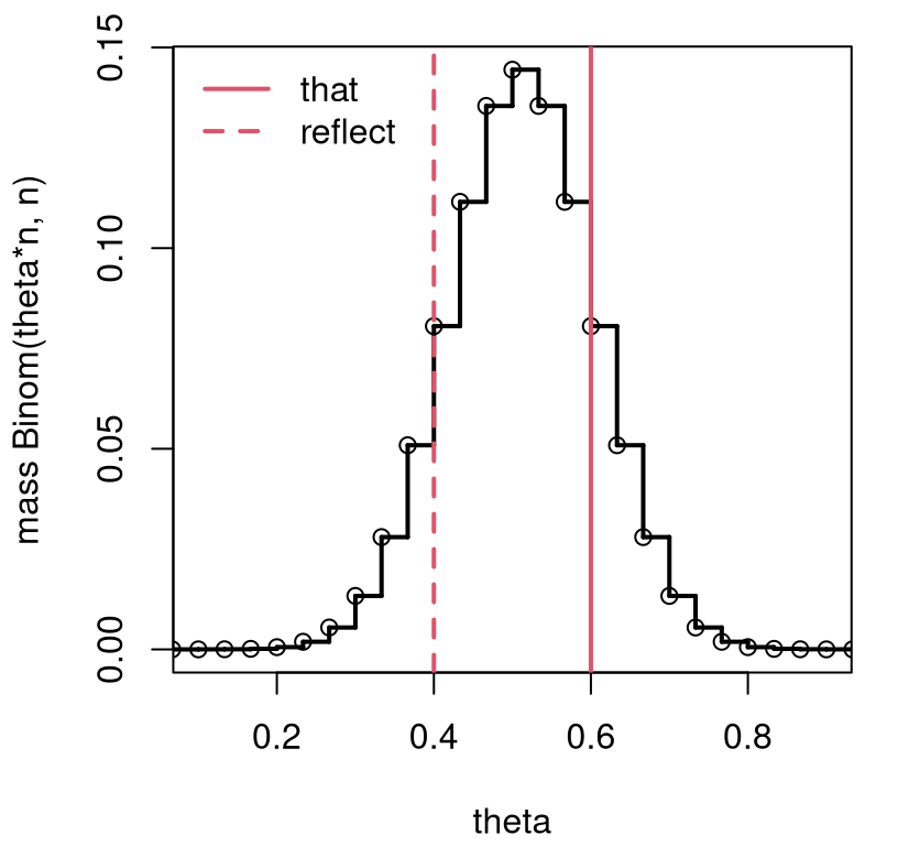

FIGURE 3.1: Exact \(\theta = \frac{1}{2}\) sampling mass characterizing the distribution for \(S_n\) corresponding to a Bernoulli/binomial analysis of coin flips from Chapter 1.

Observe how this view is similar to the one from Figure 1.1, so the conclusion will be similar, too. A \(p\)-value adds precision. This is easier to express as a sum over possible \(s_n\)-values, since those are integers, than as \(\theta\)-values. Let \(r\) denote the reflected value of \(s_n\), and \(f(s;n, \theta)\) represent the mass implied by Eq. (3.7). Then,

\[\begin{equation} \mbox{$p$-value:} \quad \psi = \sum_{s=0}^r f(y; n, \theta) + \sum_{s=s_n}^n f(y; n, \theta), \quad \mbox{where $f$ is the binomial mass}. \tag{3.8} \end{equation}\]

This assumes the statistic \(s_n\) is in the right tail, and its reflection is in the left one. The bounds of those sums are reversed if the observed statistic is in the other tail.

In R code, Eq. (3.8) goes like this. For mass functions (like the binomial), p* functions (like pbinom below) sum up masses provided by analogous d* functions (like dbinom). We’ll talk a little more in generality about this soon when we get to the Gaussian example.

pbinom(n - s, n, 0.5) + pbinom(s - 0.5, n, 0.5, lower.tail=FALSE)

## [1] 0.3616

Note that for the calculation in the right tail it’s important to subtract off something in \((0,1)\) – I did 0.5. Anything small will do. This is just a fluke of the way that the pbinom function is implemented in R. Without that, the calculation is off of what binom.test provides, which you can check against results in §1.4.

Quick digression on precision. It’s easy to be off a bit by missing little details, both here in the “math” calculation, and also when doing MC. But that doesn’t mean you’re not doing it right. Here the issue boils down to how strict inequalities (like \(<\) and \(>\)) are used in p* calculations, versus those that include \(=\) (like \(\leq\) and \(\geq\)). I try not to dwell too much on these edge cases. At the same time, I’d like to show you what’s needed to match what software libraries provide, at least as far as possible. Ideally MC calculations would match up exactly too, but there are many factors that make that difficult. One is the MC error inherent to calculations with pseudo-random numbers (§A.3). That can be mitigated with bigger \(N\). Other discrepancies can be explained by arbitrary choices (both by me and by the authors of those libraries).

The particular edge case in question here is actually more nuanced than what I have described above. The “fix” only works in this particular example, and others very similar to it. There are more such considerations – more edges – required to cover issues that arise in greater generality. I’ll show you another one in just a moment. You can have a look at how those are handled in R by inspecting the binom.test function. (Entering binom.test at the command prompt dumps the code.) Such is the beauty of open source software, although the code isn’t documented as well as I wish it was. You won’t get much of an explanation for why those adjustments are important.

Regardless, it is the process and transparency in calculations that is paramount, not the precision of the final answer. Any borderline case, like a \(p\)-value near \(\alpha = 0.05\), or any other \(\alpha\), demands greater scrutiny. That might mean collecting more data, or it might mean thinking more about how the experiment is designed, what distributions are assumed, or what the right hypotheses are. If you’re curious, I have some more thoughts along these lines in the Preface to the book.

Alright, back to our example. Whether you find that easier or harder than MC perhaps depends on if you prefer math or computing. The mathematical solution is elegant, but I think the computing version is more intuitive, as it is faithful to the experience of “what if” modeling behind hypothesis tests. From a mathematical perspective, this is about as easy as it gets. For computing, the difficulty level is “medium”. You’ll recall from Chapter 2 that just about the same code works there for Gaussian samples. You’ll see momentarily that the math for that case is more challenging.

As a final variation, consider the case of \(\mathcal{H}_0: \theta = 0.8\), as entertained with monty.bern via pval.discrete in §1.4. Recall that I described a rule determining the value of the reflected statistic, which was inspired by binom.test. Here’s that rule played out with calculations described above. We still have that \(S_n \sim \mathrm{Bin}(n, \theta)\), but now \(\theta = 0.8\). Our test statistic is the same too, \(s_n = 0.6\), but now it’s in the left tail. In R, and in pval.discrete, the reflected value is determined by the location of the largest mass point from the opposite tail (from the right) which is less than the mass corresponding to \(s_n\). That is …

ms <- dbinom(s, n, 0.8)                     ## mass of s from data
mgrid <- dbinom(sgrid, n, 0.8)              ## mass of all s in 1:n
ti <- which(sgrid > 0.8*n & mgrid <= ms)    ## all right tail w lower mass
ri <- ti[which.max(mgrid[ti])]              ## index of largest
r <- sgrid[ri]                              ## extract reflection

Figure 3.2 provides a visual of the sampling distribution, the test statistic, and its two-tailed reflection. Notice how the view is similar to Figure 1.3, but this time based on math rather than MC. (Also, the \(x\)-axis is labeled differently, for \(s_n\) rather than \(\theta\).)

sfun <- stepfun(theta[-1], c(dbinom(sgrid, n, 0.8)))
plot(sfun, xlim=c(0.5, 1), xlab="theta", ylab="mass Binom(theta*n, n)", 
  main="", lwd=2)
abline(v=c(that, r/n), lty=1:2, col=2, lwd=2)
legend("bottom", c("that", "reflect"), lty=1:2, col=2, lwd=2, bty="n")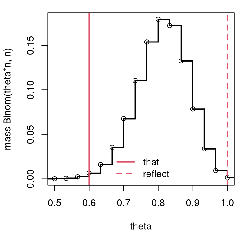

FIGURE 3.2: Exact \(\theta = 0.8\) sampling mass, otherwise following the setup in Figure 3.1.

The \(p\)-value calculation follows Eq. (3.8), but with different \(r\) and \(\theta\), and with \(r\) and \(s\) flipped because tails are reversed.

pbinom(s, n, 0.8) + pbinom(r - 0.5, n, 0.8, lower.tail=FALSE)

## [1] 0.01073

Check that this matches what was provided by binom.test at the end of Chapter 1. It’s interesting, I think, that the hard part of this test is the calculation of the reflection. Deriving (and sampling from) the sampling distribution is the easy part.

Location \(p\)-value analytically

A sum of independent Gaussians is Gaussian. This means that for \(Y_i \stackrel{\mathrm{iid}}{\sim} \mathcal{N}(\mu, \sigma^2)\), for \(i=1,\dots, n\), aggregate \(\sum_i Y_i\) is Gaussian and thus so is \(\hat{\mu} = \bar{Y} = \frac{1}{n} \sum_i Y_i\). Moreover, Gaussians are special in that their moments are in 1:1 correspondence with parameters \(\mu, \sigma^2\), and uniquely determined by those values. So if we know the mean and variance (i.e., the first and second moments), and we know that the distribution is Gaussian, then we know all we need to know to fully characterize the distribution. Regurgitating Eqs. (2.3) and (2.4), we have

\[\begin{equation} \hat{\mu} = \bar{Y}, \quad \mathbb{E}\{ \bar{Y} \} = \mu, \quad \mbox{ and } \quad \mathbb{V}\mathrm{ar}\{ \bar{Y} \} = \frac{\sigma^2}{n}. \quad \mbox{Therefore} \quad \bar{Y} \sim \mathcal{N}(\mu, \sigma^2/n). \tag{3.9} \end{equation}\]

Rehashing: we know the sampling distribution of our estimator \(\hat{\mu}\), which is the same as our chosen test statistic \(S_n \equiv \hat{\mu}\). In the Gaussian analysis of heights data from §2.2 we presumed that \(\sigma^2\) was known. We now have a way to estimate \(\sigma^2\) via MLE, but hold that thought for a moment. I’ll come back to it. For this discussion, and to make a direct contrast to what we got (by MC) in Chapter 2, it’s better to first presume \(\sigma^2\) known and keep the value we used earlier: \(\sigma^2 = 6.25\). That way, we have everything we need to make a comparison between observed \(\bar{y} = 66.62\) and its sampling distribution (3.9). Figure 3.3 has that visual.

ygrid <- seq(61.5, 67.5, length=1000)
plot(ygrid, dnorm(ygrid, mu, sqrt(sigma2/n)), type="l", 
  xlab="ybar = muhat", ylab="density N(64.5, 2.5^2/n)")
abline(v=muhat, col=2, lwd=2)
legend("topleft", "observed", lty=1, col=2, lwd=2, bty="n")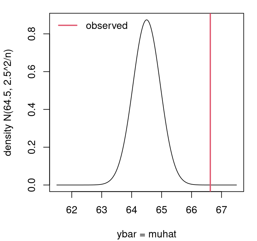

FIGURE 3.3: Exact sampling density characterizing the distribution for \(\bar{Y}\) corresponding to the Gaussian analysis of heights data from Chapter 2.

See how similar things look here compared to the MC analog in Figure 2.2. Labeling on the \(y\)-axis is different and the histogram looks more discrete, but shapes and positioning on the \(x\)-axis (which is for \(\bar{Y}\)) are similar. In both cases, the observed value of the statistic (vertical red line) is far from the bulk of the distribution, nudging us toward rejecting the null hypothesis.

Having a Gaussian sampling distribution makes it easy to be precise with a \(p\)-value calculation. We don’t need to “reflect” the observed statistic onto the other side of the density, because Gaussians provide symmetry. Once we know the \(p\)-value for one tail, we can double it to get a two-sided value.

The mathematical way to calculate the area under a curve – like we did by summing under the histogram or masses earlier – is to integrate. Specifically in the Gaussian heights setting:

\[ \mbox{$p$-value:} \quad \psi = 2 \times \int_{\bar{y}}^\infty f(y; \mu, \sigma^2/n)\; dy, \quad \mbox{where $f$ is the Gaussian density}. \]

Note that this assumes that \(\bar{y} > \mu\) from the null hypothesis; otherwise, we must work in the left/lower tail with \(\int_{-\infty}^{\bar{y}}\) instead. The computation required is not something that can be done with pen and paper unfortunately, but it can be done numerically in R via quadrature.

ny <- length(y) ## this is n from Chap 2, clashing with binomial n
pval <- 2*integrate(dnorm, muhat, Inf, mean=64.5, sd=sqrt(sigma2/ny))$value
pval

## [1] 3.125e-05

Be aware that sigma2 was set in Chapter 2. Notice that this is exactly the same value we got from the z.test in §2.4. In a way, our MC alternative can be seen as a form of quadrature. MC integration is a topic in and of itself, but largely for another book.

For important distributions like the Gaussian, R has a built-in way to numerically integrate densities. In fact, you may recall from a first class in probability that such an integral (or sum) is known as cumulative distribution function (cdf). Each generating function in R, beginning r* like rnorm, has a density version d* like dnorm, and a cdf version beginning with p* like pnorm. We can do:

2*pnorm(muhat, 64.5, sqrt(sigma2/ny), lower.tail=FALSE)

## [1] 3.125e-05

By default, pnorm and other cdf functions in R prefer to integrate in the lower tail, from \(-\infty\) to the statistic \(\hat{\mu}\), which is how a cdf is usually defined. But if you provide lower.tail=FALSE, they instead do \(\hat{\mu}\) to \(\infty\).

So why is this called a \(z\)-test? Because \(z\) is the letter people have settled on for standard normal deviates: \(Z \sim N(0, 1)\). Back in the day, textbooks included “\(z\)-tables” in the back so you could look up \(p\)-values (cdf evaluations) under a standard Gaussian and other distributions. Some still do, but I think that’s old-fashioned now that we have R. Before you could use one of those tables for your particular test, you had to calculate a \(z\) statistic, sometimes called the standard score. The standard score centers and re-scales your \(\hat{\mu} \equiv \bar{y}\) under the null hypothesis by subtracting off mean \(\mu\) and dividing by standard deviation \(\sqrt{\sigma^2/n}\).

\[\begin{align} z &= \frac{\bar{y} - \mu}{\sigma/\sqrt{n}} & \quad &\mbox{with} \quad & Z &\sim \mathcal{N}(0,1) \tag{3.10} \end{align}\]

The quantity in the denominator \(\sigma/\sqrt{n}\), which is the square root of the variance of the estimator, has a special name: standard error or “se”. When viewing \(\bar{y}\) as a random quantity \(\bar{Y}\), we obtain a standard Gaussian \(Z\).

One way to view a \(z\) statistic, and many of the other test statistics I shall introduce later, is: estimate (“\(\mathrm{est}\)”) minus “want to know” (“\(\mathrm{wtk}\)”) divided by standard error.

\[\begin{equation} \mathrm{stat} = \frac{\mathrm{est} - \mathrm{wtk}}{\mathrm{se}} \tag{3.11} \end{equation}\]

The “\(\mathrm{wtk}\)” comes from the null hypothesis. Here is the \(z\) statistic for our heights analysis.

se <- sqrt(sigma2/ny)
z <- (muhat - 64.5)/se
z

## [1] 4.164

One nice thing about a \(z\) statistic, especially if you don’t love looking up old-school tables, is that you can do a quick-and-dirty check by comparing to \(\pm 2\). If \(z\) is bigger than two in absolute value, then reject \(\mathcal{H}_0\) at the \(\alpha = 0.05\) level. Alas, about 95% of a Gaussian density likes within \([-2, 2]\).

Paired with \(z\) is another special letter, now in Greek: \(\phi(y) \equiv f(y; \mu = 1, \sigma^2=1)\). The integral of that density is \(\Phi(z) = \int_{-\infty}^z \phi(y)\; dy\) so that

\[\begin{equation} \mbox{$p$-value:} \quad \psi = 2 \times \Phi(-|z|). \tag{3.12} \end{equation}\]

The minus absolute-value part ensures a left-tail calculation, and \(2\times\) makes it two-tailed by symmetry. If you took stats in the 20th century, you would look up \(-|z|\) in a \(\Phi\) table, but with R we can use its built-in numerical integration capability.

2*pnorm(-abs(z))

## [1] 3.125e-05

Same as before. An interesting side-fact, however, is that pnorm uses a table lookup to some extent, leaning on pre-computed “quadrature supports” that can be quickly linearly interpolated. I thought you’d like to know. At least you don’t have to do it; the computer does it for you. If you were a really clever undergrad in the 20th century you’d photocopy the table in the back of the book so that you didn’t have to keep flipping back and forth. What are you going to do with all the time freed up by not having to do all that?

Infamous \(t\)-test

Brace yourself. This is going to be a long, but important “example”.

You may have found it unsatisfying to fix \(\sigma^2\). Our hypothesis test (2.2) focused on the location parameter \(\mu\), but since we also used a fixed \(\sigma^2\) value in the analysis – whether in Chapter 2 or just above in the previous example – we were implicitly folding a value of \(\sigma^2\) into the null hypothesis. Ideally, \(\mathcal{H}_0\) would focus only on what’s important. If only \(\mu\) is of interest, our calculations should be agnostic to anything else, like \(\sigma^2\).

I just showed you how to estimate \(\sigma^2\), via MLE (3.5) or after bias correction (3.6). Let’s stick with the latter going forward. Yet with focus on \(\mu\), it’s not ideal to just “plug-in” \(s^2\) everywhere that \(\sigma^2\) is used. Two reasons: (1) \(\hat{\mu} = \bar{y}\) is buried in \(s^2\), so we’re using the same info twice; (2) \(s^2\) is just the setting that makes the observed data most probable, modulo bias correction. There are many other settings that could explain the data (almost) as well. It would be better to use \(s^2\) for \(\sigma^2\) in a way that acknowledges that a diversity of values are plausible, and that also compensates for the presence of \(\hat{\mu}\) within \(s^2\).

Quick digression. I’m not aiming for a sampling distribution for \(s^2\). We’ll look at things like that later, in Chapter 6, when testing for variances is of interest. Quantity \(\sigma^2\) is a nuisance, not a main object of inquiry in this chapter. I want to make it vanish, in a sense. The statistical way to do that is to marginalize it out by averaging over all plausible values. I wish I could show you the Bayesian version, which would be more natural, but that’s a whole different book.

Alright, back to what we are going to do. I’ll teach you a little about sums-of-squares under a Gaussian distribution, which isn’t too bad, and I’ll wave my hands audibly when we get to the hard part. There’s a very important result here that I want to get to, because I need to use it lots in the book. I’ll use it even while avoiding math in favor of MC. It’s so fundamental. Perhaps the most unsatisfying bit here is that we’re going to do a lot of work, but it’s not (usually) going to result in a different outcome. The reason for that is coming later in §4.1. But we’ll feel better that we’re making a full accounting of uncertainty. Or at least I will.

Ok, here we go. A really important identity that’s clearly relevant to our discussion is written in the equation below. You might not have thought of it on your own, but it’s not that hard to show. So I’ve left it for you as a homework exercise.

\[\begin{equation} \sum_{i=1}^n \frac{(Y_i - \mu)^2}{\sigma^2} = \frac{(n-1)s^2}{\sigma^2} + \frac{(\bar{Y} - \mu)^2}{\sigma^2/n} \tag{3.13} \end{equation}\]

This is useful for two reasons. One is that it relates quantities we don’t know, or don’t want to commit to (\(\sigma^2\)), to those that can be calculated from data (\(s^2\)). The other is that (I’ll show you) we know the distributions of two out of the three terms, so we can use that to deduce the third. Here we go.

If \(Y_i \sim \mathcal{N}(0,1)\), then \(Y_i^2 \sim \chi^2_1\) where \(\chi^2_\nu\) is a chi-squared (\(\chi^2\)) distribution with \(\nu\) degrees of freedom (DoF). This isn’t something I need to prove to you. Think of it as a definition. Someone worked out some hard math to derive the density for \(Y_i^2\) when \(Y_i\) is a standard Gaussian and decided to name it after a Greek letter. Go figure. I’m not going to show you the density function, because it’s not important to what we’re doing. You could easily simulate from a \(\chi^2\). Just draw \(Y_i \sim \mathcal{N}(0,1)\) and square it. It’s easier to use rchisq directly, and we’re going to do that in just a moment. Before that, I want to generalize things a little.

The first way is pretty simple: if \(Y_i \sim \mathcal{N}(\mu, \sigma^2)\) then \((Y_i - \mu)^2/\sigma^2 \sim \chi_1^2\). After standardizing, you get the standard normal result. Look back at the final term in Eq. (3.13). Since \(\bar{Y} \sim \mathcal{N}(\mu, \sigma^2/n)\), I get to use this result immediately.

\[\begin{equation} \frac{(\bar{Y} - \mu)^2}{\sigma^2/n} \sim \chi_1^2 \tag{3.14} \end{equation}\]

One way to interpret this, that’s useful for understanding later, is that \(\bar{Y}\) is worth one DoF (\(\nu = 1\)). That’s one “piece of information”, after all the \(y_i\)’s are added up. I think of DoF as PoI, but I’m not going to use that acronym because I’m not that cavalier. I’ll stick to DoF.

Here is the second generalization I promised you. If you have \(Y_1, \dots, Y_n \stackrel{\mathrm{iid}}{\sim} \mathcal{N}(0,1)\), then \(\sum_{i=1}^n Y_i^2 \sim \chi^2_n\). You can consider this to be an extension of the definition of \(\chi^2_\nu\) that I talked about above. Basically this means you can add up \(\chi_1^2\)’s, accumulating DoF. And if we have \(Y_1, \dots, Y_n \stackrel{\mathrm{iid}}{\sim}\mathcal{N}(\mu,\sigma^2)\) more generally, then

\[\begin{equation} \sum_{i=1}^n \frac{(Y_i - \mu)^2}{\sigma^2} \sim \chi_n^2. \tag{3.15} \end{equation}\]

So \(Y_1, \dots, Y_n\) are worth \(n\) DoF; \(n\) pieces of information. That makes sense. Eqs. (3.14) and (3.15) provide two of the three terms in Eq. (3.13), so we can solve for the last one through “additivity” of \(\chi^2\)’s. Referring back to Eq. (3.13),

\[ \chi^2_n = \left[ \chi^2_{n-1} \right] + \chi^2_1, \]

where the term in brackets is the one we’re looking for. This is where, technically speaking, I’m waving my hands a little because proving that is beyond our reach. That’s why “additivity” is in quotes. In case you’re curious, the result is a consequence of Cochran’s theorem. The key part of it, in brackets, can be rearranged to give the result we need about \(\sigma^2\) by solving across the \(\sim\) as if it were an \(=\):

\[\begin{equation} \frac{(n-1)S^2}{\sigma^2} \sim \chi_{n-1}^2 \quad \Rightarrow \quad \sigma^2 \sim \frac{(n-1)s^2}{\chi_{n-1}^2}. \tag{3.16} \end{equation}\]

In other words, \(n\) pieces of information is equal to \(n-1 + 1\) pieces of information. Burying \(\bar{y}\) inside \(s^2\) costs one DoF because those data, \(y_1, \dots, y_n\), appear twice: once as each \(y_i\) and once as \(\bar{y}\). The \(\chi^2_{n-1}\) for \(s^2\), after some scaling, corrects (or accounts for) this double-use by subtracting of one DoF for \(\bar{y}\).

Figure 3.4 illustrates how the distribution for \(\sigma^2\) in Eq. (3.16) compares to \(s^2\). I use a sample of \(\sigma^2\) values, and form an empirical distribution via histogram. That sample will be reused momentarily to expand our \(z\)-test.

sigma2s <- (ny - 1)*s2/rchisq(N2, ny - 1)
hist(sigma2s, main="", xlim=c(0, 20))
abline(v=c(s2, sigma2), lty=1:2, col=2, lwd=2)
legend("topright", c("s2", "sigma2"), lty=1:2, col=2, lwd=2, bty="n")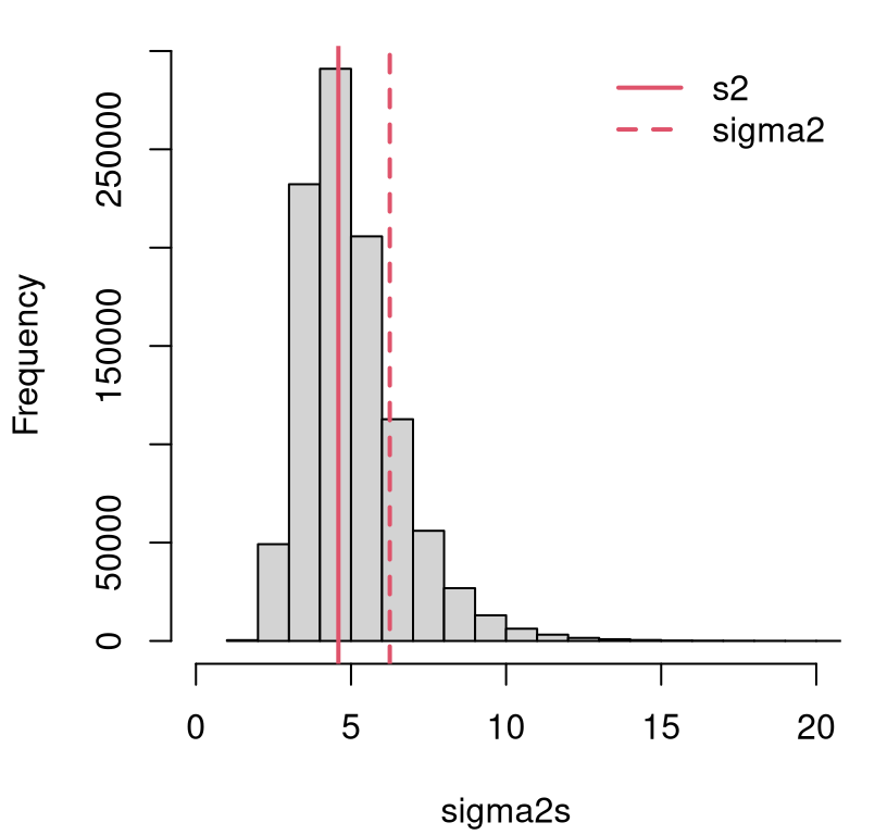

FIGURE 3.4: Distribution for \(\sigma^2\) in the heights example from Chapter 1.

Quantity \(s^2\), indicated by the solid red vertical line, is just the “central” value. There are many other nearby settings (both smaller and larger) that are reasonable. The same can be said for the value of \(\sigma^2\) (dashed red line) used for the test in §2.2, tacitly part of \(\mathcal{H}_0\). Using just one setting – any setting, but especially ones in the left tail of the distribution – will undercut any assessment of uncertainty about the main quantity of interest: \(\mu\). The value of \(\sigma^2\) that I fixed for convenience in Chapter 2.2 is bigger than a substantial proportion of sampled \(\sigma^2\) values.

mean(sigma2s < sigma2)

## [1] 0.8138

It may have been overly conservative; we were overestimating uncertainty in that analysis, although that doesn’t take into account the values as large as twenty (or larger) in the right-hand tail in Figure 3.4. But there’s no reason to wonder when we can do! It’s easy to use these samples as part of the MC from §2.3.

Ss <- rep(NA, N2)                   
for(i in 1:N2) {  
  ## sigma2s[i] <- (ny - 1)*s2/rchisq(1, ny - 1)   ## if not done above
  Ys <- rnorm(ny, mu, sqrt(sigma2s[i]))            ## only real change here
  Ss[i] <- mean(Ys)                     
}

I’m not going to show you a histogram of those samples, because it looks very similar to Figure 2.2. But check out the \(p\)-value calculation.

pval <- mean(Ss < 2*mu - muhat) + mean(Ss > muhat)  ## muhat=s from Ch 2
pval

## [1] 6.8e-05

Indeed, we get a smaller \(p\)-value because, on the whole, we’re using smaller values of \(\sigma^2\) now than earlier. What would happen with a \(z\)-test with \(s^2\) plugged in instead? This time, I’ll hit the easy button and use a library.

z.test(y, mu=mu, sigma.x=sqrt(s2))$p.value

## [1] 1.187e-06

Notice how this value is quite a bit smaller. Using \(s^2\), while central, misses accounting for the possibility of much larger \(\sigma^2\) values under its \(\chi_{n-1}^2\) distribution.

Accounting for all reasonable \(\sigma^2\) values in a \(z\)-test yields a \(t\)-test and, like the \(z\)-test, that name will take some explaining. An English statistician named William Sealy Gosset, who worked as head brewer for Guinness, published a paper about some of the work he was doing for his employer under the pseudonym Student. Some of that work was about the form of Gaussian random variables sampled under a chi-squared variance. Specifically, Gosset was interested in

\[\begin{equation} f_t(y) = \int_0^\infty f_\phi(y; \mu, \sigma^2) \times f_{\chi^{-2}} (\sigma^2; \nu) \; d \sigma^2, \tag{3.17} \end{equation}\]

where \(f_\phi\) is the density of \(\mathcal{N}(\mu, \sigma^2)\) and \(f_{\chi^{-2}}\) is the \((n-1) s^2\) scaled inverse-\(\chi_\nu\) from Eq. (3.16). The technical term for forming a density by integrating over one of its parameters as a random effect is called convolution. By sampling \(\sigma^2\) values and plugging them into a Gaussian generator, tens of thousands of times and then averaging, we have implemented a MC integral by convolution.

Gosset showed that the solution to this integral has an analytic closed form, and \(f_t(y)\) is now known as the (density of the) Student-\(t\) distribution. (Some say “Student’s-\(t\)”, but I think that’s harder to verbalize and to write.) Using the form suggested by Eq. (3.17), this distribution has parameters: \(\mu\) specifying location or mean, \(\sigma^2\) for scale, and DoF \(\nu\). Together \(\nu\) and \(\sigma^2\) determine the variance of the random variable. Synthesizing \(Y \sim \mathcal{N}(\mu, \sigma^2)\) and \(\sigma^2 \sim (n-1)s^2/\chi_\nu^2\), one might write \(Y \sim \mathrm{St}(\nu; \mu; s^2)\). I’m not going to bore you with the mathematical form of its density, since we don’t need it for anything, but I will help you visualize it momentarily.

Like in a \(z\)-test, which uses a standardized Gaussian statistic, a \(t\)-test uses the Student-\(t\) in standardized form: \(T \sim t_\nu \equiv \mathrm{St}(\nu; 0, 1)\) via:

\[\begin{align} t &= \frac{\bar{y} - \mu}{s^2/\sqrt{n}} & \quad &\mbox{with} \quad & T &\sim t_\nu. \tag{3.18} \end{align}\]

Notice how that follows the same generic test statistic setup as in Eq. (3.11): same estimate \(\hat{\mu}\), same value \(\mu = 64.5\) from \(\mathcal{H}_0\), but different standard error \(\sqrt{s^2/n}\). Viewing \(\bar{Y}\) as a random quantity yields random \(T\) which is distributed as \(t_\nu\).

Contrasting a Gaussian with a Student-\(t\) is subtle. Figure 3.5 provides a visual based on standardized versions. Two variations on \(t_{\nu}\) are provided. One, in dashed red, sets \(\nu = n - 1\) with particular \(n\)-value taken from our heights analysis (\(n = 24\)). The other shows \(\nu=5\), a more exaggerated DoF.

ztgrid <- seq(-5, 5, length=1000)
plot(ztgrid, dnorm(ztgrid), type="l", xlab="z or t", 
    ylab="density N & St", lwd=2)
lines(ztgrid, dt(ztgrid, ny - 1), lty=2, col=2, lwd=2)
lines(ztgrid, dt(ztgrid, 5), lty=2, col=3, lwd=2)
legend("topright", c("Gauss", paste0("St_nu=", ny - 1), "St_nu=5"), 
  lty=1:3, col=1:3, lwd=2, bty="n")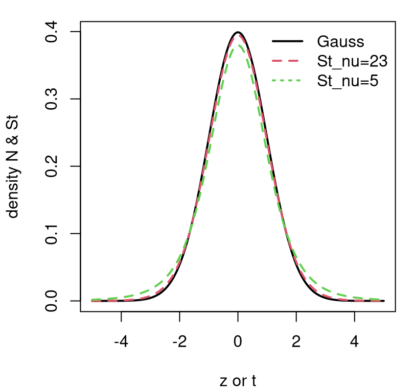

FIGURE 3.5: Contrasting \(\phi\) and \(t_{\nu = \{23, 5\}}\) densities.

Observe how a Student-\(t\) has lower density for central values, near zero, and higher density in its tails. This is especially so when the DoF parameter \(\nu\) is small, but it’s also true in general for any \(\nu\)-value. Eventually, however, as \(\nu > 30\) or so, it’s really hard to tell the difference between a \(t_\nu\) distribution and a Gaussian one. But with a small data set – a small \(n\) – there could be a big difference. Since that difference manifests as heavier tails, a test based on a Student-\(t\) sampling distribution generally provides a more conservative (i.e., larger) \(p\)-value, making one less likely to reject \(\mathcal{H}_0\). It always yields a larger \(p\)-value compared to a \(z\)-test with \(\sigma^2 = s^2\) plugged in.

Another way to contrast Gaussian and Student-\(t\) distributions is to look at their 95% quantiles.

q <- c(0.025, 0.975)                   ## central 95% is 2.5% and 97.5%
rbind(gauss=qnorm(q), t=qt(q, ny-1))

##         [,1]  [,2]
## gauss -1.960 1.960
## t     -2.069 2.069

The \(t_\nu\) gives a wider 95% interval because it has heavier tails. But notice that, at least for \(\nu = 23\), they both hover about the same amount around \(\pm 2\). So like with \(z\)-tests, \(|t| > 2\) makes for a good threshold to quickly test a statistic and decide on \(\mathcal{H}_0\) without bothering with a \(p\)-value.

Here’s what we get for the \(t\)-test on the heights data.

se <- sqrt(s2/ny)           ## same as z, but with sigma2 = s2
t <- (muhat - 64.5)/se      ## same as z, different se above
t

## [1] 4.858

Like with the \(z\)-test, this is an easy reject. But, just to check that everything lines up with our earlier, MC setup, I’ll finish with a \(p\)-value calculation. Again, symmetry of the Student-\(t\) simplifies a two-tailed integral.

pval.exact <- 2*pt(-abs(t), df=ny - 1)
pval.exact

## [1] 6.638e-05

Notice that this is very close to the MC alternative introduced first. That number is repeated below, along with the result from R’s built-in t.test library function.

c(mc=pval, exact=pval.exact, lib=t.test(y, mu=mu)$p.value)

##        mc     exact       lib 
## 6.800e-05 6.638e-05 6.638e-05

Now you know how to do a \(t\)-test, perhaps the most famous (or infamous) statistical test there is. It’s really the same thing as a \(z\)-test, but averaging over the distribution of variances \(\sigma^2\), rather than just plugging one in.

3.3 Confidence intervals

A confidence interval (CI) can be thought of as the inverse of a hypothesis test. Let \(\hat{\theta}\) generically denote an estimate (e.g., MLE) for a parameter \(\theta\) of interest. Suppose you were to pick an \(\alpha\) such that you would reject \(\mathcal{H}_0: \theta = \theta_0\) if your \(p\)-value satisfied \(\psi(\theta_0, \hat{\theta}) < \alpha\). Then a CI is defined by the following set

\[ \mathrm{CI} = \{ \theta_0 : \psi(\theta_0, \hat{\theta}) \geq \alpha \}. \]

Said another way, a CI contains all values \(\theta_0\) such that \(\psi(\theta_0, \hat{\theta}) > \alpha\), i.e., \(\theta_0\)’s for which you would not reject \(\mathcal{H}_0\). The bounds of that interval, which are what usually gets reported, can be identified by \(\psi(\theta_0, \hat{\theta}) = \alpha\).

Technically that is just one definition of a CI; there are others which are less directly related to \(p\)-values. The one I’ve described is a central CI consistent with a two-sided hypothesis test. Perhaps the biggest issue with that definition is that it doesn’t immediately tell you how to calculate one. As might not surprise you, I’m going to give you two ways: (1) by MC, which always works; and (2) one using math, which is sometimes doable, and sometimes not so much.

You can form a central CI (or just CI going forward) by revisiting the MC for a hypothesis test and plugging in the estimate of the parameter of interest \(\hat{\theta}\) for the null \(\theta\). Use that value to simulate new \(\tilde{\theta}(Y_1, \dots, Y_n)\)’s, calculated in the same way as \(\hat{\theta}\) from the observed data, just with simulated observations. Once you’re done with the simulation, report the lower \(q_{\alpha/2}\) and upper \(q_{1-\alpha/2}\) empirical quantiles of that sample. So if you take \(N=10{,}000\) MC samples and \(\alpha = 0.05\), report the 250th smallest and 250th largest (9,750th smallest) samples of \(\hat{\theta}\) as your 95% CI.

I think that verbal description is sufficient and that we don’t need a formal Algorithm environment, especially if I augment with a couple of examples.

Toss up CI via MC

First for \(\theta\) in the coin-flipping experiment.

thats <- rep(NA, N)                      
for(i in 1:N) {                       
  Ys <- rbinom(n, 1, that)               ## use that=ybar instead of theta
  thats[i] <- mean(Ys)                   ## use Ybar
}
CImc.theta <- quantile(thats, c(0.025, 0.975))
CImc.theta

##   2.5%  97.5% 
## 0.4333 0.7667

The explanation here, or for any CI, is that there’s a 95% chance that the true, but unknown \(\theta\) value is inside this interval: \([0.43, 0.77]\). That is, when you make an interval like this 100 times, with 100 different observed data sets, about 95 of them will contain the true \(\theta\). We say that there’s a 95% chance that the CI covers the true value of the parameter. There’s a little caveat, here, that I’ll delve more into when we discuss the closed-form version, momentarily. If you prefer, you can explain the CI in the context of a hypothesis test. For any value of \(\theta\) lying inside CI, we would fail to reject \(\mathcal{H}_0\); for any value outside, we could reject at the specified \(\alpha\) level.

Location CI via MC

Here the focus is on \(\mu\) from the Gaussian heights example. I’ll skip straight ahead to the full variance-integrated (3.17) version of the sampling distribution behind the \(t\)-test. We’ll come back to \(z\)’s later. Cutting-and-pasting that MC with minor modification …

muhats <- rep(NA, N2)                   
for(i in 1:N2) {  
  Ys <- rnorm(ny, muhat, sqrt(sigma2s[i]))    ## use muhat instead of mu
  muhats[i] <- mean(Ys)                     
}
CImc.mu <- quantile(muhats, c(0.025, 0.975))
CImc.mu

##  2.5% 97.5% 
## 65.72 67.53

So there’s a 95% chance that the true, but unknown \(\mu\) lies inside: \([65.72, 67.53]\). For any value of \(\mu\) lying inside CI, we would fail to reject \(\mathcal{H}_0\).

---

How do you calculate a CI analytically, using math rather than simulation? Well, that can be both more difficult, or easier depending on the situation. There’s no generic approach like with MC. Everything is on a case-by-case basis. It turns out that the two cases we’ve been playing with so far have exact solutions that aren’t too hard to work out.

More widely, many CI constructions are based on asymptotics, which is the subject of Chapter 4. This involves reducing calculations to approximations based on Gaussian distributions and \(z\) statistics. So pay close attention when we get to the location CI example, because we’ll be reusing that again later, and lots.

But first, coin flips. Actually, the standard CI for \(\theta\) in a Bernoulli experiment is based on asymptotics, and I’ll show you that later. I’ve always found strange that this is the case, because it can be done exactly in closed form.

Toss up CI analytically

Eq. (3.7) says that sums \(S_n \sim \mathrm{Bin}(n, \theta)\). So just plug in \(\theta = \hat{\theta}\), extract 2.5% and 97.5% quantiles of that distribution, and divide them by \(n\) to get an interval for \(\theta\). The quantile function is the inverse of the cdf. Give it a probability, and it’ll return the value of the cdf that achieves that probability.

CI.theta <- qbinom(c(0.025, 0.975), n, that)/n
rbind(mc=CImc.theta, exact=CI.theta)

##         2.5%  97.5%
## mc    0.4333 0.7667
## exact 0.4333 0.7667

This is identical to what we got by MC earlier. But it’s not exactly the same as what R provides.

CI.theta.R <- as.numeric(binom.test(s, n)$conf.int)
CI.theta.R

## [1] 0.4060 0.7734

The reason for this is alluded to, but not entirely explained by, R’s documentation for binom.test, which says (paraphrasing): CIs are obtained by a procedure first given in Clopper and Pearson (1934). I don’t know about you, but I find this to be unsatisfying, almost 100 years later. Surely there’s a better explanation.

I’ll give it a go, based on my limited understanding of the situation from other reading. One issue is that a quantile-based CI can be problematic with a discrete distribution. The distribution may not have a quantile at exactly 2.5% or 97.5%, say. This is true for our particular binomial, whose quantiles are given by the following probabilities.

ps <- pbinom(1:n, n, that)
ps[ps > 0.001 & ps < 0.999]       ## focus away from the tails

##  [1] 0.002854 0.008302 0.021240 0.048112 0.097057 0.175369 0.285496
##  [8] 0.421534 0.568910 0.708528 0.823714 0.905989 0.956476 0.982817
## [15] 0.994341 0.998490

That being the case, one might wonder what that quantile command actually provided. Which of those percentiles did it use? More importantly, did the interval actually cover 95%?

c(hand=diff(pbinom(CI.theta*n, n, that)), 
  R=diff(pbinom(CI.theta.R*n, n, that)))

##   hand      R 
## 0.9347 0.9616

Our by-hand one does not, and therefore neither does our MC one. Those are too small, but not by much. Our interval “under-covers” because the probability is below 95%. R’s is more conservative. This is just something to be aware of. It’s definitely fixable, by being more specific about the desired outcome. For example, if we said that the lower bound of the CI should be defined by the closest percentile below 2.5%, and the upper above 95%, then we could report the following.

lw <- qbinom(max(ps[ps <= 0.025]), n, that)/n
up <- qbinom(min(ps[ps >= 0.975]), n, that)/n
CI.theta2 <- c(lw, up)
CI.theta2

## [1] 0.4000 0.7667

This is much closer to R’s, but not identical. (I’ll leave it to you as an exercise to fix the MC interval similarly.) This new interval’s coverage is, interestingly, identical even though it the interval itself is slightly different.

diff(pbinom(CI.theta.R*n, n, that))

## [1] 0.9616

Clopper and Pearson (1934) must be looking at something else. Appropriate coverage is only one piece of the puzzle. If I’m being honest here, this is getting pretty advanced, and you may even feel things are going off the rails. I won’t ask you to pay this much attention to detail on your homework, but I do think it’s important to be aware of.

A real problem arises when you observe zero heads. This isn’t likely when the true \(\theta\) is near \(1/2\) and when \(n\), the number of flips, is large. But it’s not impossible. If \(n\) is small, you can get all tails in \(n=6\) flips more than one in 100 times. The trouble is that the procedure I’ve explained, either by MC or closed-form calculation, breaks down in that case because \(\hat{\theta} = 0\). Check it out.

qbinom(c(0.025, 0.975), 6, 0)/6

## [1] 0 0

Having a confidence interval span 0 to 0 is nonsense. You’d get that for any \(n\) if there were no heads. This is a situation where the math breaks down, because the sampling distribution is degenerate. It provides no reasonable percentiles.

as.numeric(binom.test(0, 6)$conf.int)

## [1] 0.0000 0.4593

Everything covers 100%. I see this as a little like the denominator problem in \(\hat{\sigma}^2\), and getting zero variance for \(n=1\). This was a problem noticed long ago, and there are several methods for correcting it. I’ll show you another one later in §4.2. Clopper and Pearson (1934) provide one way of doing that.

I’m not going to explain it to you, because it would not be a fruitful digression. But look how big that interval is. It nearly covers half of the space of possible \(\theta\)’s. Suffice it to say that the mechanism is like a hedge – a sensible one in my opinion. If you took a small sample, say a blood sample testing for human immunodeficiency virus (HIV), you wouldn’t want to conclude that HIV was non-existent in your population, with essentially zero variability, based on just a limited number of tests. You can read more about this here, and we’ll revisit some of it in §4.1 around Eq. (4.6). As long as you have some “heads”, and your \(\hat{\theta} \ne 0\), then you don’t have to worry about it.

Location CI analytically

Recall from Eq. (3.10) that \(Z = \sqrt{n}(\bar{Y} - \mu)/\sigma \sim \mathcal{N}(0,1)\) assuming \(\sigma^2\) is fixed at a known value. For any Gaussian \(Z\), we can find quantiles \(q_{\alpha/2}\) and \(q_{1-\alpha/2}\) bracketing the central \(100 \times (1 - \alpha)\)% of the distribution. That is,

\[ 1-\alpha = \mathbb{P}(q_{\alpha/2} < Z < q_{1-\alpha/2}). \]

For example …

alpha <- 0.05
q <- qnorm(c(alpha/2, 1 - alpha/2))
q

## [1] -1.96  1.96

In this particular Gaussian case, we can write \(q_p = \Phi^{-1}(p)\). Recall that the standard Gaussian cdf is notated as \(\Phi\).

Now, write \(Z = \sqrt{n}(\bar{Y} - \mu)/\sigma\), and rearrange terms on both sides of both inequalities.

\[ \begin{aligned} 1 - \alpha &= \mathbb{P} \left(q_{\alpha/2} < \frac{\bar{Y} - \mu}{\sigma /\sqrt{n}} < q_{1-\alpha/2} \right)\\ &= \mathbb{P} \left(\bar{Y} + \frac{\sigma}{\sqrt{n}} q_{\alpha/2} < \mu < \bar{Y} + \frac{\sigma}{\sqrt{n}} q_{1-\alpha/2} \right) \end{aligned} \]

So to build an interval for \(\mu\), which captures its value within its bounds \(100 \times (1 - \alpha)\)% of the time, use

\[\begin{equation} \mathrm{CI} = \left[\bar{y} + \frac{\sigma}{\sqrt{n}} q_{\alpha/2}, \bar{y} + \frac{\sigma}{\sqrt{n}} q_{1-\alpha/2}\right], \quad \mbox{ or equivalently } \quad \bar{y} \pm \frac{\sigma}{\sqrt{n}} q_{1-\alpha/2}. \tag{3.19} \end{equation}\]

The last expression works because \(-q_{1-\alpha/2} = q_{\alpha/2}\) due to symmetry.

It’s worth reiterating the right interpretation here, because it’s easy to get wrong. This interval, when we build it over-and-over again with different \(\bar{Y}\) values calculated from Gaussian \(Y_1, \dots, Y_n\), will capture the true \(\mu\) value 95% of the time if \(\alpha = 0.05\). There’s a hypothetical frequency argument behind many classical statistical methods. A MC alternative virtualizes that frequency hypothetical in computer code, actually repeating things over and over again.

Using \(\bar{y} \equiv \hat{\mu}\) from the heights example, one can build the following CI.

CIz.mu <- muhat + q*sqrt(sigma2/ny)
CIz.mu

## [1] 65.62 67.63

Notice that I don’t need the \(\pm\) here because q, calculated above, is already both positive and negative. There’s a perfect match with the library calculation.

as.numeric(z.test(y, sigma.x=sqrt(sigma2))$conf.int)

## [1] 65.62 67.63

Notice that I don’t need to specify a mu argument if I only care about the CI. The quantity \(\mu\), which is unknown (but might be a “want to know”), does not feature in Eq. (3.19). The CI is telling you what \(\mu\)’s could not be rejected as null hypotheses.

Here is a helpful, generic version of Eq. (3.11) for CIs:

\[\begin{equation} \mathrm{CI} = \mathrm{est} \pm q \times \mathrm{se}, \tag{3.20} \end{equation}\]

where “\(\mathrm{est}\)” is the estimated parameter, \(q\) is/are the quantile(s) of its distribution and “\(\mathrm{se}\)” is the standard error. You could use this with a Student-\(t\) distribution, and \(s^2\)-based standard error, in order to average over \(\sigma^2\) values. Use qt to get \(t\) quantiles similarly. I’ve left that for you as a homework exercise. Don’t forget to check your work via t.test(...)$conf.int.

You might be worried that this CI does not actually achieve 95% coverage, because I made a big deal about that with the coin-flipping example. But don’t worry, things are just fine.

diff(pnorm(CIz.mu, muhat, sqrt(sigma2/ny)))

## [1] 0.95

Bingo. Working with a continuous, and symmetric, distribution is much easier.

3.4 What is inference?

The title of this chapter is “A little math: inference”. What does that word mean?. I’m sure you can get a lot of perspectives on that depending on who you ask, whether two different statisticians, or one statistician and one machine learner. I don’t want to put my foot in my mouth on that.

I think it’s uncontroversial that statistical inference comprises at least three things: (1) dialing in parameter settings; (2) summarizing uncertainty about those parameters; and (3) parlaying estimates and uncertainties into conclusions or predictions. For (1), I like MLEs but there are plenty of other options, and many choices amount to more or less the same thing. For (2), I’m thinking both CIs and testing hypotheses. We talked about how those are related to/inverses of one another, and both amount to ruling out (or not) certain values for the unknown quantity as a function of the estimate (e.g., MLE) and its sampling distribution. For (3), it’s about establishing a causal link, or extrapolating or interpolating to novel experimental conditions. This book doesn’t have as much of that, but we will dabble from time to time, especially with prediction.

There are even more intimate connections between MLEs, confidence intervals, and hypothesis tests. These are the subject of Chapter 4. In early drafts of this book, the contents of Chapter 4 were merged with Chapter 3, because both involve techniques for inference. But I realized that a single combined chapter would simply have been too long. It makes sense to stop halfway, digest, take stock, and get practice with some exercises.

3.5 Homework exercises

These exercises help gain experience with the math and closed-form calculations behind statistical inference carried out by Monte Carlo in earlier chapters, and with \(t\)-tests and confidence intervals, which are new to this chapter.

Ensure that you are using methods outlined in this chapter. Many students will have experience working with closed-form Bernoulli/binomal tests, \(t\)-tests, and others (like Poisson, exponential, etc.) in other contexts, particularly via approximation (i.e., converting to \(z\)-tests) from previous classes, other books, or materials found online. Those will be discussed and evaluated in later chapters and homeworks. Deploying non-Chapter 3 methods here will likely not earn full credit.

Do these problems with your own code, or code from this book. In some cases you can check your work, e.g., with with t.test. However, check with your instructor first to see what’s allowed. Unless stated explicitly otherwise, avoid use of libraries in your solutions. Throughout, I suggest you keep it simple and double a one-sided \(p\)-value calculation for two-tailed tests.

#1: Poisson

Let \(Y_1, \dots, Y_n\) be iid Poisson with unknown mean \(\theta\), i.e., \(Y_i \stackrel{\mathrm{iid}}{\sim} \mathrm{Pois}(\theta)\). Use Wikipedia to find facts about this distribution, like the form its mass, etc., but the idea is to show your work. Poissons are used for counts of events that happen in a certain period of time. Note that on Wikipedia, \(\lambda \equiv \theta\) and \(k \equiv y\).

1. Derive the maximum likelihood estimator \(\hat{\theta}\) for \(\theta\). What is the sufficient statistic for \(\theta\)?
2. Derive the sampling distribution for \(\hat{\theta}\) in closed form. Hint: you may wish to use this fact about sums of Poisson random variables.

Use the data values for \(y_1, \dots, y_n\) given in R below to answer the remaining parts. These data are a count of the number of buses that stop at fifty randomly selected stops in a one-hour time period.

y <- c(3, 5, 6, 5, 2, 6, 6, 7, 8, 8, 7, 8, 0, 5, 7, 6, 6, 10, 6, 5, 6, 7, 
  6, 9, 8, 4, 8, 7, 11, 9, 4, 4, 7, 9, 8, 6, 5, 6, 12, 10, 7, 13, 8, 12, 
  9, 4, 10, 8, 4, 5)

Hint: try poisson.test(sum(y), length(y), theta), but only to check your work.

3. A city planner asserts that the typical number of buses that pass by any particular stop in a given hour is 6. Do these data support this? Use both empirical (MC) and closed-form/exact calculations. Hint: this is a hypothesis testing question.

4. Provide a (central 95%) CI for \(\theta\). Show both empirical (MC) and closed-form/exact calculations. Advanced: does your CI have appropriate coverage?

#2: Exponential

Let \(Y_1, \dots, Y_n\) be iid exponential with unknown rate parameter \(\theta\), i.e., \(Y_i \stackrel{\mathrm{iid}}{\sim} \mathrm{Exp}(\theta)\). Use Wikipedia to find facts about this distribution, like the form of the density, etc., but show your work! The exponential distribution can be thought of as the “inverse” of a Poisson: the waiting time for one thing to happen. Note that on Wikipedia, \(\lambda \equiv \theta\) and \(x \equiv y\).

1. Derive the maximum likelihood estimator \(\hat{\theta}\) for \(\theta\). What is the sufficient statistic for \(\theta\)?
2. Derive the sampling distribution for \(\hat{\theta}\) in closed form. Hint: you may wish to use a fact from here about sums of exponential random variables.

Use the data values for \(y_1, \dots, y_n\) given in R below to answer the remaining parts. These are “times-to-failure” in years obtained from an accelerated life test of a certain new smart-TV.

y <- c(3.71, 17.70, 23.49, 9.60, 16.16, 4.94, 10.69, 14.62, 11.27, 1.99, 
  10.95, 4.87, 14.87, 26.37, 0.78, 1.60, 9.21, 18.73, 18.85, 6.71, 11.45,
  4.02, 7.57, 14.75, 3.48, 10.03, 16.21, 25.94, 3.11, 17.61)

Hint: I was unable to find any appropriate add-on packages to help check work, so you’re kinda on your own with this one.

3. The TV manufacturer claims that the typical lifespan of their new smart-TV is twenty years. Do these data support this? Use both empirical (MC) and closed-form/exact calculations. (This is a hypothesis testing question.)

4. Provide a (central 95%) CI for \(\theta\), and interpret that as a CI for the number of years until failure. Show both empirical (MC) and closed-form/exact calculations.

#3: Scale-1 Pareto

Let \(Y_1, \dots, Y_n\) be iid Pareto with scale fixed at \(\beta = 1\), and unknown shape parameter \(\theta > 0\). Specifically, \(Y_i \stackrel{\mathrm{iid}}{\sim} \mathrm{Pareto}(1; \theta)\), with density \(f(y; \theta) = \theta / y^{\theta + 1}\) for \(y \geq 1\) and zero otherwise. Note that on Wikipedia, the scale is notated as \(x_m\), and I am using \(x_m = \beta = 1\). Shape is notated as \(\alpha\), and I am using \(\alpha = \theta\).

1. Derive the maximum likelihood estimator \(\hat{\theta}\) for \(\theta\). What is the sufficient statistic for \(\theta\)?

2. I’m not going to ask you to derive the sampling distribution in closed form. I think this is one that’s lots easier by Monte Carlo. But I’m giving it to you so you can compare, if curious. Malik (1970) says that \(1/\hat{\theta} \sim \mathrm{Gamma}(n-1, n\theta)\). The calculation is similar to #2b.

Use the data values for \(y_1, \dots, y_n\) given in R below to answer the remaining parts. These are insurance claims, in millions of dollars, for trucking companies operating in 2024.

y <- c(1.15, 1.26, 2.98, 1.41, 1.01, 1.16, 1.02, 1.38, 1.40, 1.20, 1.017,
 1.71, 1.91, 1.00, 1.95, 1.14, 1.29, 1.11, 1.14, 1.29, 1.06)

3. A re-insurer asserts that the mean claim in 2024 is $1.5M, which corresponds to \(\theta = 3\). Do these data support this? (This is a hypothesis testing question. The Pareto package on CRAN provides rPareto for random deviates.)

4. Provide a (central 95%) CI for \(\theta\).

#4: Sufficient statistics for Gaussian/location model

What are the sufficient statistics for the Gaussian model? Hint: there are two.

#5: Biased MLE \(\hat{\sigma}^2\)

Show \(\mathbb{E}\{\hat{\sigma}^2\} = \frac{n-1}{n} \sigma^2\), with \(\hat{\sigma}^2\) given in Eq. (3.5). You may use that \(\bar{Y}\) is unbiased for \(\mu\) and any other definitions from earlier in the chapter. Hint: start on the left-hand side, and make manipulations to arrive at the expression on the right-hand side. Use properties of expectation and variance.

#6: Sums of squares decomposition

Show (3.13). Hint: start on the left-hand side, and make manipulations to arrive at the expression on the right-hand side. A helpful first step is to replace \(Y_i - \mu\) with \(Y_i - \bar{Y} + \bar{Y} - \mu\) and then expand out the square.

#7: Update monty.bern with exact calculations

Update monty.bern from §1.4 to include the exact calculations covered in §3.2 and CI calculations from §3.3, including optional visuals. Check the N argument. Interpret N=0 as meaning no MC sampling, and in that case use exact calculations instead of MC. That way the same library function can be used for both. Test this new capability by checking that results agree on the homework questions in §1.5.

#8: Revisit Bernoulli

Revisit any of Exercises #2 (silicone wafers), #3 (PVC or copper piping), or #4 (GPS speed vs. speedometer) from §1.5, but do it the “math way” with closed-form calculations. Additionally provide CIs, checking MC simulation matches closed-form/math results. (This will be pretty easy if you already did #7 above.)

#9: Library function for \(t\)-test

Write a library function like monty.z from §2.6 but for \(t\)-tests. Call it monty.t. Implement both MC versions and closed form/exact calculations, which may be invoked when N=0 is provided. See #7 above. Include optional visuals when vis=TRUE in both cases, MC and exact, and return a similar list of relevant quantities to t.test including \(s^2\) and a CI. Test it out and make sure it works.

#10: ROI with \(t\)-test

Revisit §2.6 #5–6 with a \(t\)-test, i.e., estimate \(s^2\) and test \(\mu = \{15, 17\}\), separately. Provide a CI for \(\mu\). Use both empirical (MC) and closed-form/exact calculations (which is pretty easy if you did #9 first).

#11: One-liner

Revisit exercise #7 from §2.6 and update it to sample from a Student-\(t\) sampling distribution by replacing sigma2 with an appropriate rchisq call, producing a one-liner MC \(t\)-test. (It’ll be a long one-liner.)

References

Clopper, C. J., and E. S. Pearson. 1934. “The Use of Confidence or Fiducial Limits Illustrated in the Case of the Binomial.” Biometrika 26: 404–13.

Malik, H. J. 1970. “Estimation of the Parameters of the Pareto Distribution.” Metrika 15 (1): 126–32.

---

5. Careful not to confuse the index \(p\), counting parameters, with \(p\)-value. If I ever need to put a \(p\)-value, generically, into a mathematical expression, I will use the Greek \(\psi\) to avoid confusion.↩︎

6. Not with respect to \(\sigma\). Treat \((\sigma^2)\) as a single quantity, like \(x\), and differentiate with respect to \(x\).↩︎