Chapter 10 Pearson \(\chi^2\)-tests
I know what you’re thinking. We did \(\chi^2\)-tests back in Chapter 6. You’re right. The ones in this chapter aren’t all that different. Chapter 6’s focus was on a particular parameter, \(\sigma^2\) in a Gaussian model, or \(\sigma_y^2\) and \(\sigma_x^2\) for two samples. That was back in the land of parametric (P) statistics. This chapter’s \(\chi^2\)-tests involve a similar statistic, but they’re non-P and they’re not (usually) about variance.
Remember, testing statistics are your choice, and they need not be neatly matched to an estimated quantity. It’s convenient that residual sums of squares (RSSs) have a \(\chi^2\) distribution. We’ve used that fact a number of times, across several chapters. I won’t list them all here. Recall our discussion around Eq. (7.18) where I explained that you could estimate, and thus test, variance under a simple linear regression model by borrowing from a simple means model (3.5), writing \(\mu_i = \beta_0 + \beta_i x_i\). Here that idea is appropriated for another sort of \(\mu_i\). Both of those were Gaussian models, but it works even in a non-Gaussian setting because of the central limit theorem (CLT; §4.1). It works for any distribution, even ones without “parameters”. RSSs are highly portable.
In this chapter I’ll show you how to use normalized RSSs to test other/many aspect(s) of a distribution, in both one- and multi-sample contexts. Emphasis will be on non-P settings, although I’ll show you an important application to P testing. Closed-form versions of the tests are exclusively asymptotic, due to their connection to the CLT. With small sample sizes, \(n\), it can be hard to know whether those calculations are accurate. With Monte Carlo (MC), one can ensure that accuracy is only a question of computation effort.
10.1 Goodness-of-fit
So far, our tests have targeted specific, yet sometimes relative, features of a distribution of random quantities. Now I want to pivot to something that’s simultaneously more specific and more all-encompassing. Here focus will be on a single population having a certain distribution. Rather than scrutinize a particular aspect, like a mean, median or standard deviation, a goodness-of-fit (GoF) test looks at the entire distribution. Such a bold approach must be reigned in a little bit. Usually \(\chi^2\)-tests are on discrete and finite distributions. They’re also applicable to real-valued ones through binning. I’ll show you.
Suppose our data consist of \(n\) independent observations of a random variable \(Y\) grouped into \(c\) classes. Grouping implies that sufficient information about such data would comprise the number of observations that are sorted into each class. Let \(o_j\), for \(j=1,\dots,c\), denote those observed counts. Each must be a non-negative integer, and \(\sum_{j=0}^c o_j = n\). These quantities are often presented in a \(1 \times c\) contingency table (CT). See Table 10.1. CTs with one-dimensional rows or columns represent overkill, since you can just list observed counts in-line like \(o_1, o_2, \dots, o_c\), but we’ll see more interesting ones later, and it makes sense to start simple.
| class 1 | class 2 | \(\cdots\) | class \(c\) | total | |
|---|---|---|---|---|---|
| observed | \(o_1\) | \(o_2\) | \(\cdots\) | \(o_c\) | \(n = \sum_j o_j\) |
These data are compared against a distribution, specified as probabilities by the null hypothesis: \(p_1, \dots, p_c\), where \(p_j \geq 0\) for \(j=1,\dots,c\) and \(\sum_{j=1}^c p_j = 1\). If \(c = 2\), then those probabilities, along with \(n\), prescribe a binomial distribution like in Chapter 1 for coin flips. In that context \(o_1\) and \(o_2\) tally the number of heads and tails, respectively, in \(n\) flips. When \(c > 2\) we have what is known as a multinomial distribution, of which the binomial is a special case.
You don’t really need to know many multinomial facts to understand the basics, except moments which I shall provide momentarily. There are some shortcuts in code if you’re willing to work with a multinomial random-number generator. I’ll show it to you both ways later and other technical nuggets as needed. For now, just think of a \(c\)-sided die that you roll \(n\) times instead of flipping a two-sided coin.
Let \(p = p_1, \dots, p_c\) denote the \(c\)-vector of probabilities, and likewise let \(o = o_1, \dots, o_c\) denote observations. Then, technically speaking, the model is
\[ \mbox{Model:} \quad\quad O \sim \mathrm{Multinom}(n, p). \]
Don’t let the presence of \(O\) on the left of \(\sim\) trip you up. True, I almost exclusively have \(Y\) in that position, and sometimes \(X\), elsewhere in the book. Here, \(Y\) determines \(O\) through some classification or tally, as in Table 10.1. \(O\) is a compact way to look at \(Y\): \(o_j = \sum_{i=1}^n 1_{\{y_i = \, \mathrm{ class } \,j\}}\).
Multinomial means and variances are upgrades of results from the binomial:
\[\begin{equation} \mathbb{E}\{O_j\} = n p_j \quad \mathrm{ and } \quad \mathbb{V}\mathrm{ar}\{O_j\} = n p_j (1 - p_j) \quad \mbox{ for } \quad j=1,\dots,c. \tag{10.1} \end{equation}\]
Quick digression on notation. Throughout, I’ve been careful to use Greek letters for parameters, but here I’ve used \(p\) instead of \(\theta\), like for the binomial in Chapter 1. I could – maybe I should – but I’m sticking with \(p\) here for a number of reasons. One is that the literature prefers \(p\) for GoF and similar tests, and that’s related to my second reason. GoF tests are thought of as non-P, where the notion of “parameter” is complicated to say the least. How could a test that’s non-P involve a \(c\)-vector of unknown parameters \(\theta\)? Good question.
In a GoF test, and also for tests of independence and homogeneity coming soon in §10.3, probabilities \(p\) serve as an intermediary. They’re derived from some other distribution or relationship of interest. That distribution might involve other, genuine parameters \(\theta\), or it might not. I’ll table that for a later discussion, beginning in §10.2, so we don’t get derailed here. For now, just be aware of it and know that I know that I’m not following my own rules. I’ve given it some thought and have decided that the presentation here works best with \(p\), not \(\theta\) which will come back later.
Alright, back to inference. The formal hypotheses involved in a GoF test question whether a particular \(p\) could have generated observations \(o\). Let \(p_0\) be a specific \(c\)-vector of probabilities.
\[\begin{align} \mathcal{H}_0 &: p = p_0 && \mbox{null hypothesis (“what if")} \tag{10.2} \\ \mathcal{H}_1 &: p \ne p_0 && \mbox{alternative hypothesis} \notag \end{align}\]
Above, \(p \ne p_0\) means that any of the \(c\) probabilities could differ. Since they must sum to one, changing one probability really means changing two or more. Going forward, I shall drop the cumbersome subscript in \(p_0\) and simply refer to \(p\) under the null hypothesis. I have a particular \(p\) in mind for some reason or another and I want to know if it could have generated what was observed, \(o\). This involves studying the sampling distribution for some statistic that can be calculated for \(o\), and sampled for \(O\), under \(\mathcal{H}_0\).
Following Eq. (10.1), let \(e_j = n p_j\), denote expectations for \(j=1, \dots, c\). Again, such quantities might have been assigned Greek letters elsewhere in the book, but I’m sticking with convention here and I think it will make sense from context as we get to fancier examples. Note that \(\sum_{j=1}^c e_j = n\).
If the \(p_j\) values specified by \(\mathcal{H}_0\) are correct, then \(o_j\) should be close to \(e_j\), on average. So a sensible statistic comparing the two might aggregate their discrepancies: \(\sum_j (o_j - e_j)^2\). Pearson’s \(\chi^2\) statistic normalizes each discrepancy before aggregating.
\[\begin{equation} x^2_{nc} = \sum_{j=1}^c \frac{(o_j - e_j)^2}{e_j} \tag{10.3} \end{equation}\]
Quick digression on notation and nomenclature. You’ll see how \(\chi^2\) distributions are involved when we get more into some of the math. I’ve put a complicated \(nc\) subscript, but this is not common, and I will generally drop all subscripts to streamline things. I did that above to remind you that two types of counts are involved: the total number of observations, or rolls of the dice \(n\), and the number of classes, or die faces \(c\). Although I’ve titled this section with “GoF”, a multinomial setting and Pearson’s \(\chi^2\) statistic (10.3) are quite general. Whether to call something a GoF test, multinomial test or otherwise, depends on its application. It doesn’t really matter, as will make more sense once we see some examples. The first one is coming soon.
Alright, back to analysis. Pearson’s \(\chi^2\) statistic has a few advantages over other aggregates, measuring discrepancies between observed and expected quantities under the null. Normalizing by expected counts \(e_i\) lends some interpretability since it may be shown that
\[\begin{equation} \mathbb{E}\{X_{nc}^2\} = c - 1. \tag{10.4} \end{equation}\]
I’m leaving that to you as a homework exercise in §10.4. Just follow your nose and use Eq. (10.1) liberally. So if you have an observed \(x^2\) that is much larger than \(c - 1\) you’ll probably reject. Small \(x^2\) aren’t interesting since those support the null: observed is close to expected. Only the right-hand tail matters. Other advantages to Eq. (10.3) involve even more math, and we’ll get to those after MC.
Here’s a simple example to get us going: the dice upgrade of coin flips from Chapter 1. Suppose a six-sided die was tossed 600 times, and a count of the number of times each face (with \(1, 2, \dots, 6\) dots) came up was recorded.
##   n   c
## 600   6
That’s \(c=6\) faces or classes, \(n=600\) flips, and observed counts stored in \(o\). We wish to know if the die is fair, i.e., \(p = (1/6, \dots, 1/6)\). Is the assumption of a perfectly balanced six-sided die a “good fit” to these data? Although rolling dice is an inherently multinomial enterprise, the idea of comparing observed to expected (under any model) via categories is generic. I think this is where the idea of “GoF” comes from.
Six-hundred rolls was chosen to make it easy to calculate e by hand, which
would be 100 if the die is fair. But since we have R …
## [1] 100Now, the test statistic.
## [1] 11.18Since x2 is two times larger than the distance between its mean
(10.4), which is \(c - 1 = 5\), and the smallest possible \(x_2\)
of zero, my money is on rejecting the null (barely). No need to guess, let’s
see what the sampling distribution says.
GoF test by MC
As with coin flips, the program here involves virtual dice rolling. Under \(\mathcal{H}_0\), each roll is a uniform sample of the face values \(\{1, \dots, 6\}\). For example …
## [1] 3You don’t actually need a prob argument when \(p\) is uniform, but I wanted
to make sure you knew what to do for other \(p\). A total of \(n\) such rolls may
be obtained via replacement with simple modification. Rather than record
each of \(n\) tosses individually, it’s simpler (and sufficient) to have a
summary of how many times each face came up. The table command can do that.
This time without the redundant prob argument …
##
##   1   2   3   4   5   6
## 105  95  90 102 110  98
See how we get a \(c\)-vector, just like o. All that’s left is to put that
into a big MC loop. This code is a little on the slow side because
sample and table functions incur substantial overhead. I’ll show you a
faster, and more streamlined way to do it momentarily.
N <- 100000
X2s <- rep(NA, N)
for(i in 1:N) {
  Os <- table(sample(1:c, size=n, replace=TRUE))
  X2s[i] <- sum((Os - e)^2/e)
}
Figure 10.1 shows the empirical sampling distribution for \(X^2\) along with observed \(x_2\). No reflection this time. GoF tests are right-tailed since only large distances between observed and expected offer evidence against the null.
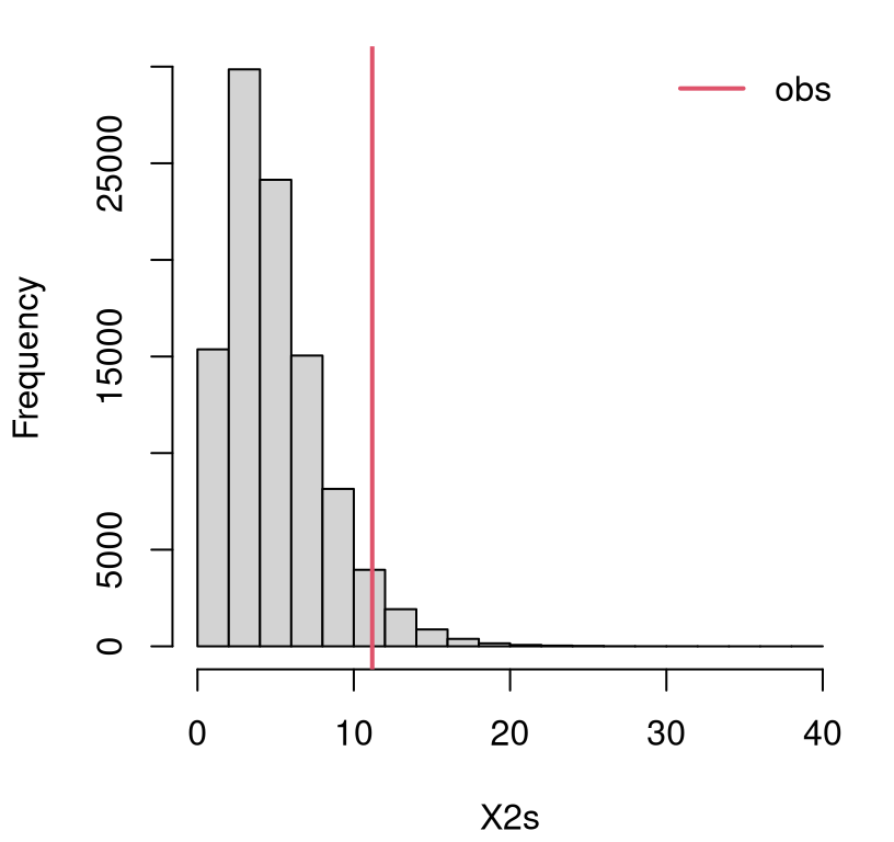
FIGURE 10.1: Empirical sampling distribution of \(X^2\) for a GoF test on dice rolls.
It’s a close call. Here is the \(p\)-value …
## [1] 0.04779… which falls on the “reject” side (this is not a fair die) of 5%. If you’re concerned you can do an even larger \(N\). I tried \(10\times\) bigger below but still saw \(\psi < 0.05\). So it’s a close call. Decisively, a reject “by the book”, but I wouldn’t bet the farm on it.
In the example above, I was deliberate in avoiding direct use or reference to a multinomial distribution. Understanding and implementing a GoF test via MC doesn’t require anything fancy, just like with coin flips in Chapter 1. Yet even in Chapter 1 it helped to recognize that counts of heads in many coin flips follows a binomial distribution. If nothing else, this streamlined MC simulation. You can play the same game here.
## [1] 101 88 92 111 106 102This time the prob argument is required. It’s not the same output as
table(sample(...)) above because random numbers are involved. But it has the
right format out-of-the-box. It’s also faster, computationally speaking.
You’re probably wondering about that drop command. This isn’t strictly
necessary, and I don’t use it in the MC loop below. What you get from
rmultinom is a matrix. Since I only asked for one sample, that matrix
is \(c \times 1\) so it takes up a lot of vertical space when printed to the
screen, or to pages of this book. The drop function will reduce the
dimension of the object in its argument if possible, in this case from a
matrix to a vector.
Here’s the new MC. We don’t really need to do it again, but I like it because it lets us explore MC error a little via \(10\times\) larger \(N\).
X2s10 <- rep(NA, 10*N)
for(i in 1:(10*N)) {
  Os <- rmultinom(1, size=n, prob=rep(1/c, c))
  X2s10[i] <- sum((Os - e)^2/e)
}
mean(X2s10 > x2)
## [1] 0.04773Observe how this agrees with previous results up to at least the first
significant digit, and is still less than 5% when rounded. Another reason
rmultinom is better than table(sample(...)) is that there’s some chance,
especially if \(n\) is large relative to \(c\), that a simulation won’t include a
representative count from all categories in \({1,\dots,c}\). When that happens,
table omits a count for those categories (which should be zero), providing a
vector on output that has fewer than \(c\) entries. The whole simulation will
break if that happens, so be aware. Using rmultinom is more robust. It
includes zero counts, so you always get a \(c\)-vector on output.
In the homework exercises of §1.5 I asked you to do a
one-liner for the binomial test. You can do that here too, but it’s
neater as a two-liner: one to calculate all \(N\times c\) samples of \(O\),
arranged in a matrix, and another to colSum the statistic. Give it a try in
§10.4.
GoF test by math
It can be shown that
\[\begin{equation} X^2_{nc} \sim \chi^2_{c-1} \quad \mbox{ as } \quad n \rightarrow \infty. \tag{10.5} \end{equation}\]
Now you know how a \(\chi^2\) distribution is involved in Pearson’s statistic. I warned you that I was just going to quote some results when it came to the math. But let me argue that this makes sense via circumstance. You already know the mean (10.4) matches exactly, and that particular result isn’t asymptotic. Variances match pretty closely too, which may be verified via MC.
##    mc  chi2
## 10.05 10.00
It makes sense that there would be \(c-1\) degrees of freedom (DoF). When \(c\) probabilities are involved, and which must sum to 1, there are really only \(c - 1\) free quantities. The last one may be determined by the others: \(p_c = 1 - \sum_{j=1}^{c-1} p_j\). Finally, we know that normalized Gaussian RSSs are \(\chi^2\), e.g., Eq. (3.15). Non-Gaussian ones enjoy similar asymptotic results via CLT. However, the CLT is for sums (or means) of \(n\) quantities not \(c\), and the limiting distribution is Gaussian not \(\chi^2\).
None of that is proof of anything, but the technical details are way outside the scope of this book. In fact, you won’t find it even in more technical books. Results like those in Eq. (10.5) come up lots, especially in non-P contexts. Measuring distance between observed and expected quantities via normalized RSS (10.3) makes sense, and those are asymptotically \(\chi^2\). Think of it like a CLT for normalized RSSs. Don’t go Googling “CLT for normalized RSSs”. You won’t find anything because I made that up, but I still think it’s a good way to remember it.
Figure 10.2 illustrates how to use that result (10.3) on the dice example, though I hope this is becoming second nature. The view is similar to the empirical sampling distribution provided by Figure 10.1.
x2grid <- seq(0, 8*(c - 1), length=1000)
plot(x2grid, dchisq(x2grid, c - 1), type="l", lwd=2)
abline(v=x2, col=2, lwd=2)
legend("topright", "obs", lwd=2, col=2, bty="n")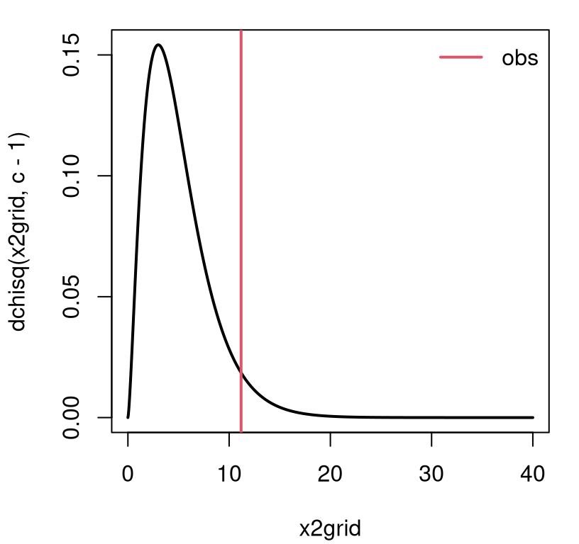
FIGURE 10.2: Asymptotic sampling distribution of \(X^2\) for GoF test on dice rolls.
A \(p\)-value calculation involves integrating into the right tail, and is in close agreement with our MC sum from earlier.
##      mc    asym
## 0.04779 0.04793
The agreement tightens with larger \(N\) in the MC. Since \(n = 600\) is large, the asymptotic approximation is probably pretty accurate, although you never can be sure.
The library function chisq.test built-into R provides an automation. All
that’s required is a vector of observed counts o. Everything it needs
is derived from o including n = sum(o) and c = length(o).
## [1] 0.04793That one matches the asymptotic result I calculated by hand above. Testing
non-uniform p requires specifying a p= argument, but that’s not absolutely
necessary otherwise since p=rep(1/length(o), length(o)) by default.
Interestingly, chisq.test has a simulate.p.value option that,
according to the documentation, provides a \(p\)-value following a MC test due
to Hope (1968). As far as I know, this is the only built-in library
function for testing simple hypotheses in R that supports MC. The
actual code for that simulation comes from Patefield (1981) and is in
Fortran. Both were way ahead of their time. Simulation was not popular in top
statistics journals even as late as the 1990s. Computing was a different
beast in 1968.
That’s it. Now you know how to perform a GoF test, or a Pearson \(\chi^2\) test. As I’ve hinted, one (GoF) is technically a special case of the other (Pearson \(\chi^2\)), but it’s a subtle distinction depending on application. You’ll see what I mean as I take you through more examples, beginning in the next section.
Operationally speaking, both are multinomial tests. Much of our analysis – especially the MC – circumvented multinomials except to make a conceptual connection. I’ve left a homework exercise to help convince you that you know how to work with multinomials. A multinomial connection makes everything seem parametric (P), but I’m presenting this in the non-P part of the book. It’s a matter of perspective. Let me show you.
10.2 P or non-P?
Rolling dice is pretty basic. Here are two more involved examples that I think will help demonstrate the capabilities of a GoF test, and also clarify the way in which it’s non-P, even though it may be applied in a P context. Larry Wasserman put GoF tests in his All of Statistics book, not his All of Non-parametric Statistics book. So it’s definitely in a gray area. Inspecting the probabilities of a few categories via expectations is not really non-P, is it? I think it depends on how few a few is, and where those probabilities come from.
Is it Gaussian?
Like, is it cake?
Data in nels_math.csv on the book webpage comes from a 2002 (national) Educational Longitudinal Study (ELS) involving a survey of students’ math scores from a sample of schools across the United States. I became aware of this data while studying Peter Hoff’s book titled A First Course in Bayesian Statistical Methods (Hoff 2009). In that book Hoff provides several variations on the analysis of these data, and all of them are based on Gaussian distributions. Is that reasonable? Let’s take a look.
nels <- read.csv("nels_math.csv")
y <- nels[nels[,1] == 1, 2]         ## math scores in first school only
n <- length(y)
n
## [1] 31We won’t handle the entire data set here, just the scores for students in the first school. There are 100 schools in total, so there’s a lot of data to play with. Each row corresponds to a student, and each entry/column records that student’s school, math score, and socio-economic status (SES), a measure of affluence for the family that student belongs to. Ignore that last column for now, too. However, an interesting subject of inquiry might be to see if there’s any association between SES and score (Chapters 7 and 12).
When entertaining a model based on a certain distribution, like a Gaussian, it helps to be specific about which Gaussian. What settings for \(\mu\) and \(\sigma^2\)? MLEs, or bias-corrected analogs, are nice and automatic and have good properties.
Now the question is more specific: is this Gaussian a good fit?
Quick digression on scope. You can do this with other distributions (with any parameters \(\theta\)), not only Gaussian. Call it a reference distribution \(\mathcal{F}\) if you want to be generic. Gaussian is a good place to start.
You may be familiar with other tools designed to assess GoF. Two visual options are provided in Figure 10.3, based on a simple histogram (left) and quantile-quantile (QQ) plot. Both offer a comparison between empirical and theoretical distributions. If you’re not really sure what a QQ-plot is, that’s fine. I’m not going to totally derail us to explain that one here. Visual tools are powerful. But here my focus is on providing a statistical test, something quantitative and methodical. From a certain perspective, statistical tests and other procedures may be seen as merely automating, and lending precision and mathematical/scientific heft to, visual checks and other judgment calls from data.
par(mfrow=c(1, 2))
ygrid <- seq(ybar - 3*sqrt(s2), ybar + 3*sqrt(s2), length=1000)
hist(y, freq=FALSE, main="", xlim=range(ygrid))
lines(ygrid, dnorm(ygrid, ybar, sqrt(s2)), col=2, lty=2, lwd=2)
legend("topright", "MLE Gauss", col=2, lty=2, lwd=2, bty="n")
qqnorm(y, main="")
qqline(y, col=2, lwd=2)
summary(dnorm(ygrid, ybar, sqrt(s2)))
## Min. 1st Qu. Median Mean 3rd Qu. Max.
## 0.00039 0.00282 0.01149 0.01476 0.02672 0.03546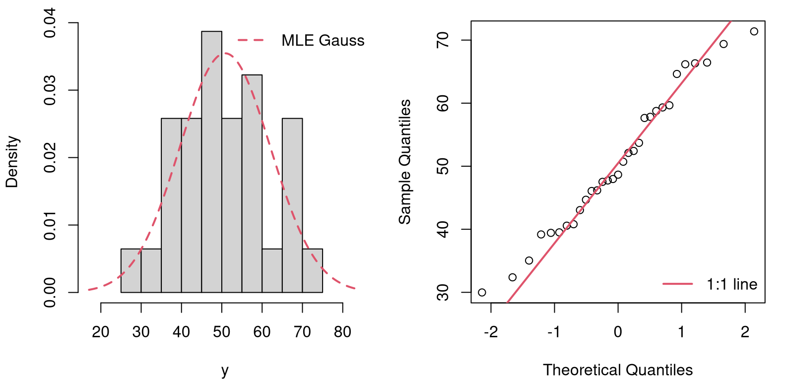
FIGURE 10.3: Visual checks of GoF of a Gaussian to the (N)ELS math data for school one: histogram (left) and QQ-plot (right).
From the figure, it’s a close call. The histogram of the raw data (left panel) is in the same “ballpark” as the estimated Gaussian – that’s the job of the MLE! – but the tails look “light” to my eye. There’s that strange dip in the 60-65 range. The QQ-plot shows a similar divergence at the tails, though it indicates less concern elsewhere. Both judgments, while rooted in visuals that have clear statistical justification, are ultimately qualitative.
A GoF test can add precision, procedure and formalism to a determination that a particular distribution offers a good fit to observed data. If the fit is good, any downstream assessments based on that distribution, such as confidence intervals (CIs) or \(t\)-tests, etc., which leverage that particular distributional form can be trusted. If the fit is bad, then any conclusions based on the assumed distribution are suspect. Either choose a different distribution, or go fully non-P.
Alright, back to testing. We have a hammer: a test based on categories. And so we need to turn our problem nail: make our data fall into categories that can be matched with probabilities and expectations. There are many ways to do that. Here’s one I came up with, which is probably not very different from other things you’d find elsewhere.
Create ten evenly spaced bins from the smallest to the largest value in the training data.
c <- 10
bins <- seq(min(y), max(y), length=c + 1)  ## c + 1 endpoints give c bins
mids <- bins[-11] + diff(bins)/2           ## for visuals later
My choice of ten is somewhat arbitrary. It’s desirable to have several observations in each bin, so you can’t have too many bins if you only have 31 data points, as with math scores observed for one school. If you have more data you can have more bins, loosely speaking. Having the bins be equally spaced also makes sense, but can be tinkered with if desired, as I’m about to do next.
Gaussians have real-valued support \((-\infty, \infty)\), so it will help to change the outermost bins to reach out to the edge of the universe.
Next, calculate the probability of a data point falling in each bin according to the reference distribution, which is Gaussian in our example. The probability for a bin with ends \((a, b)\), say \(p_{ab}\), could be calculated as a difference in (cumulative) distribution via the cdf:
\[\begin{align*} p_{ab} &= \Phi\left(\frac{b - \mu}{\sigma} \right) - \Phi\left(\frac{a - \mu}{\sigma} \right) && \mbox{ for Gaussians,} \\ \mbox{or} \quad p_{ab} &= \mathcal{F}(b) - \mathcal{F}(a) && \mbox{ generically.} \end{align*}\]
Here’s that in code for all \((a,b)\) provided by bins. At the same time, the
loop tallies a count of the number of observed points in each bin from y.
o <- p <- rep(NA, c)
for(i in 1:c) {
  p[i] <- pnorm(bins[i + 1], ybar, sqrt(s2))
  p[i] <- p[i] - pnorm(bins[i], ybar, sqrt(s2))
  o[i] <- sum(y < bins[i + 1] & y >= bins[i])
}
Figure 10.4 offers a visual of those bins, probabilities and
observations. Bin probabilities look a little wonky at the tails because (a)
these data don’t fit the distribution well out there; and (b) from
stretching to \(\pm \infty\). Recall that the bins were determined by the
observed data extremes. Try not to be bothered by the 4.25* in the code.
Probabilities (always in \([0,1]\)) and densities (always non-negative) are not
on the same scale, so I re-scaled the Gaussian density for my visual.
sfun <- stepfun(c(bins[-c(1,c + 1)]), p)
plot(sfun, xlab="y", ylab="bins & truth", main="",
  xlim=range(ygrid), ylim=c(0, 0.16), lwd=2)
lines(ygrid, 4.25*dnorm(ygrid, ybar, sqrt(s2)), col=2, lty=2, lwd=2)
text(mids, rep(0.02, length(mids)), o)
text(23, 0.02, "o:")
legend("topleft", "p", lwd=2, bty="n")
legend("topright", "MLE Gauss", col=2, lty=2, lwd=2, bty="n")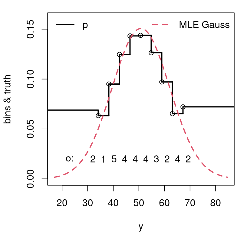
FIGURE 10.4: Visualizing classes categorized by binning an estimated Gaussian for NELS math scores.
In spite of wonky-looking probabilities in the “tail bins”, there’s reasonably
good agreement between observed bin counts, our o, and those probabilities
p. These may be readily converted into expected counts e. Calculating
Pearson’s statistic and subsequent testing may commence.
Below, find our MC from much earlier (§10.1).
Next comes \(p\)-value calculations, including by MC, math and a library
subroutine. For some reason the library gives a warning if you simply call
chisq.test(o). I’m not sure why that is. Perhaps with small \(n\) and \(c\)
there’s worry that a \(\chi^2\) approximation (10.5) is inaccurate.
You already know that I worry about that all the time! This is exactly what
MC simulation is for, and so I decided to give simulate.p.value=TRUE a try.
c(mc=mean(X2s > x2), math=pchisq(x2, c - 1, lower.tail=FALSE),
  lib.mc=chisq.test(o, p=p, simulate.p=TRUE)$p.val)
## mc math lib.mc
## 0.8832 0.8740 0.8841In any case, everyone agrees. I cannot reject the null that a Gaussian is reasonable for these data. Peter Hoff is breathing a sigh of relief – as if! By the way, his is a wonderful entry-level book on Bayesian stats – way ahead of its time blending code with serious methodological exposition, and an inspiration for many of my tutorials and books, like this one.
What really just happened? A very parametric fit – a Gaussian, the most vanilla of all ice creams – was sliced and diced with a mandoline and investigated under a multinomial microscope. Both are very “P” procedures. Parameters were estimated for one model, \(\theta = (\mu,\sigma^2)\) for the Gaussian, and used to derive parameters \(p\) for the other. But I want you to think about it as non-P because of the mandoline.
The bigger the training data size \(n\), the finer the mandoline can be, yielding larger numbers of classes, \(c\). Any modeling apparatus whose DoF, which in this case is \(c\), can grow and thereby organically refine its resolution on the data-generating mechanism, is considered non-P. You could say GoF tests are non-P because they leverage large DoF, if that helps you remember. Some setups have this in the extreme, like with ranks whose DoF grows identically with \(n\). Neural networks, especially deep ones, and kernel-based methods utilize DoF that grow faster than \(n\). Crazy, right? Some of the most advanced methods in use today are non-P.
While on the topic of DoF, notice that my GoF procedure on the Gaussian uses the data twice: once to estimate parameters \(\hat{\theta} = (\hat{\mu}, s^2)\), and then again to calculate the test statistic (10.3). Double-dipping like that usually costs you some DoF in a \(\chi^2\) sampling distribution. See discussions in Chapters 3, 5, 6, 7. This is becoming old hat. If the dimension of \(\theta\) is \(p\), then \(X^2 \sim \chi^2_{c - p - 1}\) by deduction.
It turns out this is mostly correct. On the one hand, it’s really splitting hairs. The \(\chi^2\) sampling distribution (10.5) is already an asymptotic result that is only accurate for large \(n\). In all likelihood, once \(n\) is “large enough” subtracting off a few extra DoF won’t change things much. If you want to get really technical, Chernoff and Lehmann (1954) show that the actual asymptotic distribution lies “somewhere in between” a \(\chi^2\) with \(c-p-1\) and \(c-1\) DoF. That’s not super helpful, except as justification to do whatever you feel like.
Hardy–Weinberg equilibrium
Here’s one of my favorite examples of all time, even though I know little about genetics. Others like it too; it’s a classic! Many of the initial applications of Pearson’s statistic are from genetics, coinciding with a boom of untested theories around the time of the original paper (Pearson 1900) at the turn of the 20th century. More on that with exercises in §10.4.
Consider alleles “A” and “a” with population frequencies \(1-\theta\) and \(\theta\) respectively. Under random mating, the Hardy–Weinberg (HW) principle provides that, in equilibrium (i.e., no external forces such as natural selection or mutation) expected genotype frequencies are \((1-\theta)^2\) and \(\theta^2\) for homozygotes “AA” and “aa” and \(2\theta(1-\theta)\) for heterozygotes “Aa”.
In a sample from Hong Kong in 1937, blood types occurred with the following frequencies.
## [1] 3 1029Does this follow the HW law?
Before jumping in, let’s unpack that a little. HW are basically handing us a multinomial with \(c=3\) classes, but one whose probabilities are determined by an unknown parameter \(\theta\). The question asks if these blood type data “fit” or follow a HW law. That question may be answered statistically by determining if a multinomial is a good fit for some parameter \(\theta\).
What parameter \(\theta\)? The best one, of course! So this example is a bit of a hybrid between the previous two. With dice, “nature” provides \(c\) classes and our “want to know” directly furnishes probabilities. There are no unknown parameters. With math scores, a “mandoline” provides \(c\) classes, and the Gaussian provides a probability model and unknown parameters \(\theta = (\mu, \sigma^2)\) to estimate. Here, with HW, everything is coupled together. “Nature” provides \(c=3\) classes, HW provides multinomial probabilities \(p=((1-\theta)^2, 2\theta(1-\theta), \theta^2)\), but they’re determined up to an unknown parameter \(\theta\). Rather than maximize the likelihood for \(\theta\) offline, like with the Gaussian, it must be done inline with the multinomial.
Maximizing the likelihood for \(\theta\) requires a multinomial mass function, which I’ve been avoiding until this point. If \(O \sim \mathrm{Multinom}(n, p)\), then
\[\begin{align} \mathbb{P}(O_1 = o_1, O_2 = o_2, \dots, O_c = o_c) = f(o_1,o_2,\dots,o_c; p) \tag{10.6} \\ = \binom{n}{o_1 \, o_2 \, \cdots \, o_c} p_1^{o_1}p_2^{o_2}\cdots p_c^{o_c}. \notag \end{align}\]
Notice how that generalizes the binomial (1.3), although at that time in Chapter 1 I didn’t use the word “binomial”, and I dropped the ugly normalizing combinatorial coefficient:
\[ \binom{n}{o_1 \, o_2 \, \cdots \, o_c} = \frac{n!}{o_1! o_2! \cdots o_c!}. \]
You’re more experienced now, so I can explain that this constant is technically necessary to ensure that probability masses for \(o\) add up to 1. Showing you involves writing out \(c\) nested sums, so I’ll skip that here. As in Eq. (1.3), a fully-normalized mass (10.6) is often written proportionally as
\[ f(o_1,o_2,\dots,o_c; p) \propto \prod_{j=1}^c p_j^{o_j}. \]
This is legit because the combinatorial coefficient is constant with respect to probabilities \(p = (p_1, \dots, p_c)\), and those are the main object of interest. Multiplicative constants become additive when logged, and then they vanish in the derivative, which is the next step in maximizing the likelihood (Alg. 3.1). So that coefficient wasn’t necessary in the \(c=2\) binomial case in §3.1, and nor is it here. Now I get to provide you another look at that calculation, but for \(c=3\) and \(p=((1-\theta)^2, 2\theta(1-\theta), \theta^2)\). Let’s go!
Below, \(\propto\) means there’s a dropped multiplicative constant in the case of the likelihood, and a dropped additive one in the case of its logarithm. That happens a couple of times, so be careful!
\[\begin{align*} L(\theta) &\propto ((1-\theta)^2)^{o_1} (2\theta(1-\theta))^{o_2} (\theta^2)^{o_3} \\ \ell(\theta) = \log L(\theta) % &\propto % 2 o_1 \log(1-\theta) + o_2 \log(2\theta(1-\theta)) + 2 o_3 \log\theta \\ &\propto 2 o_1 \log(1-\theta) + o_2 \log \theta + o_2 \log(1-\theta)) + 2 o_3 \log\theta \\ &= (2 o_1 + o_2)\log(1 - \theta) + (o_2 + 2o_3)\log\theta. \\ 0 \stackrel{\mathrm{set}}{=} \ell'(\theta) &= - \frac{2 o_1 + o_2}{1-\theta} + \frac{o_2 + 2o_3}{\theta} \\ % 2\theta o_1 + \theta o_2 &= o_3 - \theta o_2 + 2 o_3 - 2\theta o_3 \\ \theta (2o_1 + 2o_2 + 2o_3) &= o_2 + 2o_3 \\ \hat{\theta} &= \frac{o_2 + 2o_3}{2(o_1 + o_2 + o_3)} \end{align*}\]
Using o in R.
## [1] 0.4247The as.numeric(...) part above isn’t essential. I like it because it strips
away the names (“M”, “NM”, and “M”) I assigned to the components of o, and
which I shall put back momentarily. Plugging in gives \(\hat{p} =
((1-\hat{\theta})^2, 2\hat{\theta}(1-\hat{\theta}), \hat{\theta}^2)\).
##      M     MN      N
## 0.3310 0.4887 0.1804
That’s everything required for the GoF test. Cut-and-paste from here on out … I hope you don’t mind if I lump everything into one big code block. (It’s really not much code.)
e <- phat*n
x2 <- sum((o - e)^2/e)
for(i in 1:N) {
  Os <- rmultinom(1, size=n, prob=phat)
  X2s[i] <- sum((Os - e)^2/e)
}
c(mc=mean(X2s > x2), math=pchisq(x2, c - 1, lower.tail=FALSE),
  lib=chisq.test(o, p=phat)$p.val)
## mc math lib
## 0.9832 0.9839 0.9839Those are all basically the same and a resounding failure to reject the null. It seems that the HW principle is good to go for blood types in Hong Kong.
10.3 Homogeneity and independence
Pearson \(\chi^2\)-tests are generic. I keep repeating that, in part to apologize for not showing you all variations and applications. (I left you one in the homework.) Anywhere you can compare observed to expected, broken down into a discrete and finite number classes, a \(\chi^2\) statistic offers you a non-P test based on a multinomial.
Here I’m going to cover two very similar tests, known as the (Pearson \(\chi^2\)) test for independence and homogeneity, respectively. They’re almost the same test. In the classical/math way they are operationally identical, meaning you do exactly the same procedure but interpret the situation and results differently. This is a bit of a fudge, but any closed-form analysis is approximate via asymptotic results anyways. When using MC you can faithfully virtualize a distinction between the two setups. In spite of that, they still tend to come out about the same.
I plan to take some liberties with the presentation here in an attempt to cover two, similar things at once without being overly pedantic. Basically, I’m going to be even less formal than usual, and I hope you won’t mind. Both tests involve data that may be summarized in an \(r \times c\) CT.
Pearson’s test for homogeneity can be thought of as an \(r\)-fold upgrade to the multinomial/GoF procedure at the start of the chapter. See Table 10.2. Instead of one population sorted into \(c\) classes or categories, there are \(r\) populations. Rather than comparing classification(s) to a particular distribution, as specified by \(\mathcal{H}_0\), they are compared to one another on relative terms.
| class 1 | class 2 | \(\cdots\) | class \(c\) | total | |
|---|---|---|---|---|---|
| pop 1 | \(o_{11}\) | \(o_{12}\) | \(\cdots\) | \(o_{1c}\) | \(n_1 = \sum_j o_{1j}\) |
| pop 2 | \(o_{21}\) | \(o_{22}\) | \(\cdots\) | \(o_{2c}\) | \(n_2 = \sum_j o_{2j}\) |
| \(\vdots\) | \(\vdots\) | \(\vdots\) | \(\ddots\) | \(\vdots\) | \(\vdots\) |
| pop \(r\) | \(o_{r1}\) | \(o_{r2}\) | \(\cdots\) | \(o_{rc}\) | \(n_r = \sum_j o_{rj}\) |
| total | \(c_1=\sum_i o_{i1}\) | \(c_2=\sum_i o_{i2}\) | \(\cdots\) | \(c_c=\sum_i o_{ic}\) | \(n = \sum_{ij} o_{ij}\) |
Think of it as a classification-based ANOVA (6.3). The “want to know” is if each population (rows of the table) has the same classification probabilities as the others, or not. Specifically \(\mathcal{H}_0: O_{ij} \sim p_j\) for all \(i=1,\dots, r\), \(j=1,\dots,c\). \(\mathcal{H}_1\) that there’s some \(k \ne i\) such that \(O_{ij} \sim p_{ij}\) and \(O_{kj} \sim p_{kj}\) and \(p_{ij} \ne p_{kj}\). In other words, the null specifies that classification probabilities are the same across the rows; alternative says some are not.
Just like in a GoF test, the number of samples from each population, \(n_i\) for \(i=1, \dots, r\), is fixed by design. I mean, by the design of the experiment. The number that falls in each class \(O_{ij}\), and the total for each class \(C_j\) for \(j=1,\dots, c\) are random (with particular values observed, and represented in lowercase, in the data). Observe that \(n = \sum_{j=1}^c c_j = \sum_{i=1}^r n_i\). A tally of the last row and column totals converges on the same number.
A test for independence is different, but it has nearly the same table. See Table 10.3. The innards of the table, involving each \(o_{ij}\), are the same and to draw attention to that I’ve left those entries blank. Look at Table 10.2 for those. The final, “total” row of the table(s) is the same too, but I duplicated that part for symmetry. The thing that’s different – and it’s subtle! – is in the row totals. Those are now notated as \(r_i\) rather than \(n_i\). Also notice that I’ve renamed the rows and columns as simply “row \(i\)” and “col \(j\)”. What’s the deal?
| col 1 | col 2 | \(\cdots\) | col \(c\) | total | |
|---|---|---|---|---|---|
| row 1 | \(\cdots\) | \(r_1 = \sum_j o_{1j}\) | |||
| row 2 | \(\cdots\) | \(r_2 = \sum_j o_{2j}\) | |||
| \(\vdots\) | \(\vdots\) | \(\vdots\) | \(\ddots\) | \(\vdots\) | \(\vdots\) |
| row \(r\) | \(r_r = \sum_j o_{rj}\) | ||||
| total | \(c_1=\sum_i o_{i1}\) | \(c_2=\sum_i o_{i2}\) | \(\cdots\) | \(c_c=\sum_i o_{ic}\) | \(n = \sum_{ij} o_{ij}\) |
Tests for independence involve a single population where each individual sampled from that population is sorted by two categorizations. The CT generically notes these as “row” and “col”, respectively, of which there are \(r\) and \(c\) classes. A crucial distinction here is that row totals \(R_i\) are not fixed by the experimental design; they’re random. Although particular values \(r_i\) are observed for particular data, we would not presume to know in advance how things would be sorted by either categorization (both \(C_j\) and \(R_i\) are random).
The “want to know” is if these two classifications are dependent on one another. (The null is always the simpler option, that they are independent.) It’s not that they have the same probabilities, but rather: does knowing a row class determine what the col class is, or vice versa? The null assumes that it does not.
This is super subtle, and sometimes it’s not clear which situation is appropriate. As a practitioner, you must decide if you have separate populations across the rows, and a single classification, or one population and two classifications. I’ll give you two examples momentarily, but first we need to talk about estimation.
The “model” behind both tests is multinomial: \(O \sim \mathrm{Multinom}(n, p)\). I put model in quotes because this is really just a choice of convenience. Most would regard the procedure as non-P because the number of DoF – the number of probabilities \(p\) in the multinomial – is large. There’s one for each \(o_{ij}\) entry in the table, so the dimension of \(p\) is \(r \times c\). In that sense there isn’t really a data-generating mechanism at all, just some probabilities that may or may not depend on the row/col distinction under the null hypothesis.
Although the tables and null hypotheses for the two tests are different, the probabilities in play, and how those translate into expected counts and compare to observed counts via the test statistic, are the same. Under both nulls, rows are distinct from columns, where “distinct” either means different or independent, respectively. Consequently, both sets of probabilities for \(O_{ij}\) use \(p_{ij}\) via the following formula. Under the null …
\[\begin{equation} p_{ij} = \frac{n_i}{n} \times \frac{c_i}{n} \quad \mbox{ or } \quad \tag{10.7} p_{ij} = \frac{r_i}{n} \times \frac {c_i}{n}, \quad \mbox{ for } \quad i=1,\dots, r \, \mbox{ and } \, j=1, \dots,c, \end{equation}\]
… depending on the test. Those formulas are really the same since \(r_i \equiv n_i\); it’s just a difference of labeling. Eq. (10.7) encodes that there’s no interaction between rows and columns beyond multiplying their marginal probabilities together, as observed in the data. In this way, there aren’t actually \(r \times c\) free parameters under the null hypothesis. There are \(r + c\), since those column and row marginals determine all of the probabilities through their product. Recall that the definition of independence is that the joint factorizes as a product of marginals.
Combining Eqs. (10.7) and (10.1) gives that
\[\begin{equation} \mathbb{E}\{O_{ij}\} = n p_{ij} = \frac{n_i c_j}{n} \quad \mbox{ or } \quad \tag{10.8} \mathbb{E}\{O_{ij}\} = \frac{r_i c_j}{n}, \end{equation}\]
for all \(i\) and \(j\) as usual. Again, these two options are operationally identical. Finally, the test statistic is simply a double-sum upgrade of Person’s \(\chi^2\) from earlier (10.3):
\[\begin{equation} x^2 = \sum_{i=1}^r \sum_{j=1}^c \frac{(o_{ij} - e_{ij})^2}{e_{ij}}. \tag{10.9} \end{equation}\]
To help make these and other aspects concrete, I shall introduce two running examples, one for each test. You can probably make a case for either test being appropriate from a certain perspective, but I’ll try to make a particular argument in favor of each one.
The first came from a survey that a company did of its employees’ job satisfaction. The population is stratified by seniority from fewer than 10 years in service, to more than 40, in spans of ten. A Likert scale was used to record satisfaction with categories “miserable”, “discontent”, “content”, “happy” and “smitten”. Responses are summarized by observed count data provided below.
o <- rbind(
    c(2, 6, 20, 12, 6),
    c(4, 6, 20, 14, 7),
    c(2,  12,  28, 30, 11),
    c(1, 2, 18, 22, 12),
    c(2, 3, 4, 6, 8))
colnames(o) <- c("miser", "discon", "content", "happy", "smitten")
rownames(o) <- c("<10y", "10-20y", "20-30y", "30-40y", ">40y")
The way I’ve described it, a test for homogeneity is appropriate since there are five populations (along the rows) and five classes (columns). Those populations are not random since they’d be the same no matter what question was asked, e.g., if they were asked instead what they chose to eat for lunch. Here are the marginal totals.
Purely for aesthetics, I like to build a table in R that looks like Table 10.2. This puts the totals calculated above in an additional row and column, and displays them in a pretty format with a caption. See Table 10.4.
tab <- rbind(o, c)
tab <- cbind(tab, c(n, ntot))
colnames(tab) <- c(colnames(o), "n")
rownames(tab) <- c(rownames(o), "c")
kable(tab, caption="Job satisfaction contingency table.")| miser | discon | content | happy | smitten | n | |
|---|---|---|---|---|---|---|
| <10y | 2 | 6 | 20 | 12 | 6 | 46 |
| 10-20y | 4 | 6 | 20 | 14 | 7 | 51 |
| 20-30y | 2 | 12 | 28 | 30 | 11 | 83 |
| 30-40y | 1 | 2 | 18 | 22 | 12 | 55 |
| >40y | 2 | 3 | 4 | 6 | 8 | 23 |
| c | 11 | 29 | 90 | 84 | 44 | 258 |
The test statistic (10.9) may be calculated through expectations
(10.8). Your instinct might be to deal with double-indexing via nested
for loops like this.
e <- matrix(NA, nrow(o), ncol(o))
for(i in 1:nrow(o)) {
  for(j in 1:ncol(o)) {
    e[i,j] <- n[i]*c[j]/ntot
  }
}
There’s nothing wrong with that from a correctness perspective. I don’t like
it because it’s a clunky chunk of code, and it’s slow. Any time in R that you
need for loops for simple arithmetic, it’ll be much slower than a vectorized
alternative. Fortunately, R has an automation for exactly this kind of
calculation, which is known as an outer
product, whose binary operator
is \(\otimes\). The \(r \times c\) matrix of expectations may be abstracted as
\(\mathbb{E}(O) = n \otimes c / n\) or \(\mathbb{E}(O) = n
\otimes r / n\) depending on the test/notation. Technically, an outer product
is linear algebra, but all
that really means is “abstracted sums of products”, and those aren’t that
scary.
## [1] 0Since the sum of squared differences is numerically zero, these must be the
same quantities. It doesn’t matter which of e or efast is used below,
except in a MC where a faster and simpler code has obvious advantages. Code
below uses these to set up the test statistic. Even though a matrix e is
stored, a single vectorized sum command works transparently over both
dimensions.
## [1] 20.21The second example is based on data that could potentially generate a whole suite of examples, and you’ll have the opportunity to play with others in the exercises of §10.4. The file assault.csv contains county records on more than 5,000 assaults over a span of several years. The spreadsheet has several columns that would be interesting to analyze with the methods in this section.
Consider a table built from the location of the reported incident, and the income of the victim.
o2 <- table(assault$locale, assault$income)
o2 <- o2[,c(1,3,4,2)]   ## change column order for increasing income
o2
##
## <50K 50-75K 75-150K >150K
## rural 367 196 76 41
## suburban 905 839 480 463
## urban 1131 597 221 187My thinking here is that assault events are random, and so their location and whom they are perpetrated on (and whether or not they choose to report them) is also random. You may quibble with this, but if you allow me to press ahead, this means a test for independence is appropriate. We wish to know if income is independent of locale, and vice versa.
As earlier, I need to collect the relevant statistics and may additionally wish to construct the full table for visualization. See Table 10.5.
r2 <- rowSums(o2)
c2 <- colSums(o2)
ntot2 <- sum(r2)
tab2 <- rbind(o2, c2)
tab2 <- cbind(tab2, c(r2, ntot2))
colnames(tab2) <- c(colnames(o2), "r")
rownames(tab2) <- c(rownames(o2), "c")
kable(tab2, caption="Assault victims contingency table.")| <50K | 50-75K | 75-150K | >150K | r | |
|---|---|---|---|---|---|
| rural | 367 | 196 | 76 | 41 | 680 |
| suburban | 905 | 839 | 480 | 463 | 2687 |
| urban | 1131 | 597 | 221 | 187 | 2136 |
| c | 2403 | 1632 | 777 | 691 | 5503 |
Expectations (10.8) and test statistic via outer product (10.9) wrap up the calculations here before turning to their sampling distribution.
## [1] 271.3This time I’m going to do things in the opposite order: first math then MC. Why? Because we already know how to do it the math way, and so that’ll be really quick. MC involves a slightly bigger code than usual and so will take a little more effort, and require additional discussion.
Homogeneity/Independence via Math
We use the Pearson \(\chi^2\) statistic, the same asymptotic sampling distribution, but a different DoF. Multinomial probabilities (10.7) are calculated as an outer product of \(r-1\) (row) and \(c-1\) (column) freely estimated quantities. Recall that the “last” row and column probability is not “freely estimated” since it’s always fixed at one minus the sum of all the others. Although the table of \(e_{ij}\)-values is filled with \(r \times c\) numbers, they’re based on \((r-1) \times (c-1)\) probabilities. Therefore,
\[\begin{equation} X^2_{nrc} \sim \chi^2_{(r-1)(c-1)} \quad \mbox{ as } \quad n \rightarrow \infty. \tag{10.10} \end{equation}\]
I know this is a little hand-wavy, but it’s intuitive as an extension of
Eq. (10.5), and the math is absolutely bonkers. A \(p\)-value
may be calculated by hand, or with the same chisq.test library in R
as follows. First for job satisfaction …
pval.asym <- pchisq(x2, (nrow(o) - 1)*(ncol(o) - 1), lower.tail=FALSE)
pval.lib <- suppressWarnings(chisq.test(o)$p.value)
c(asym=pval.asym, lib=pval.lib)
## asym lib
## 0.211 0.211I put suppressWarnings(...) around the library command, because otherwise it
warns that the “Chi-squared approximation may be incorrect”. Of course, this
is always true. But the reason for the warning in this instance is that at
least one of the expected counts is less than five, a threshold built into the
software.
## [1] 1.9612 2.1744 3.5388 2.3450 0.9806 2.5853 3.9225Using simulate.p.value=TRUE is another option, and one directly comparable to
my own MC coming momentarily.
## [1] 0.2109This is not much different. It seems that there’s not enough evidence to reject the null. This was a homogeneity test, so the conclusion is that job satisfaction does not seem to vary by seniority with the company.
Now, for assaults… This time there are no warnings that require suppression.
pval2.asym <- pchisq(x22, (nrow(o2) - 1)*(ncol(o2) - 1), lower.tail=FALSE)
pval2.lib <- chisq.test(o2)$p.value
round(c(asym=pval2.asym, lib=pval2.lib), 10)
## asym lib
## 0 0This is an easy reject. Apparently, the distribution of assaults is not independent across locale and income.
Homogeneity/Independence via MC
Although mutinomials are clearly involved, and might be helpful in virtualizing random generation of \(r \times c\) tables, I prefer to begin by thinking about how raw data might be generated. By that, I mean \(n\) pairs of samples. In a test for homogeneity, row sums are fixed under the null. This means that the first of each of those \(n\) pairs is fixed. R code below generates such values for the job satisfaction example by pasting \(n_1\) ones, \(n_2\) twos, etc., up to \(n_r\) copies of \(r\).
In an actual data record these could be randomly re-ordered, but that doesn’t matter since the model assumes that those \(n\) draws are iid. Any order is fine. The other member of each pair comes from a distribution, and our best guess for those probabilities is \((c_1/n, \dots, c_c/n)\). Here’s code that generates \(n\) of those according to that distribution.
I don’t want to waste space by printing all those pairs onto the pages.
Anyways, I don’t need those values directly, just their CT summary. Because
of how the table command in R works, it’s risky to directly calculate
table(ns, Cs). If any of the random Cs values are missing full
representation of all classes, then the resulting table won’t have the right
dimensions. It could be missing entries that should be recorded as zero. The
way around that is to use a factor type to expressly provide all class
labels via its levels argument.
##    Cs
## ns   1  2  3  4  5
##   1  2  4 18 18  4
##   2  3  4 16 16 12
##   3  3 13 29 23 15
##   4  0  9 12 26  8
##   5  0  0  8 10  5
Omitting this factor step may still work for you on the examples here, but
it won’t work in all settings, and for all random MC samples. I
added them here because my code would occasionally break without them.
So that’s one random sample from the virtual data-generating mechanism under the null hippopotamus, summarized as a CT. Now I just need to do that \(N\) times, calculate expectations (10.8), and evaluate Pearson’s statistic (10.9).
for(i in 1:N) {

  ## sample under the assumption of homogeneity (null hypothesis)
  Cs <- sample(1:length(c), ntot, prob=c/ntot, replace=TRUE)

  ## build observed sample table
  Cs <- factor(Cs, levels=1:length(c))
  Os <- table(ns, Cs)

  ## build expected sample table
  ## (could also use Es <- e here)
  Es <- outer(rowSums(Os), colSums(Os)/ntot)

  ## Pearson test statistic
  X2s[i] <- sum((Os - Es)^2/Es)  ## could be NA if any Es = 0
}
Notice the parenthetical “## (could also use Es <- e here)”. The
simulation, as written, is faithful to the data-generating mechanism and the
procedure used to evaluate the test statistic. However, simulated \(O\)
values come from the same probabilities used to calculate expectations
(10.8). While each individual Es will not be identical to e, on
average they should be the same, and so it doesn’t matter which is used in the
calculation of the testing statistic via MC. I suggest trying it both ways.
How does the \(p\)-value compare to those calculated earlier? One downside to
having a random Es in the denominator is that this could result in undefined
values if any are zero. Hence the na.rm=TRUE option.
pval.mc <- mean(X2s > x2, na.rm=TRUE)  ## guard against rare Es = 0
c(mc=pval.mc, libmc=pval.libmc, asym=pval.asym, lib=pval.lib)
## mc libmc asym lib
## 0.2083 0.2109 0.2110 0.2110All are quite similar. This is one of those comparisons which is hard to narrate
since the outcome is highly sensitive to the pseudo-random numbers involved.
One explanation may be that simulate.p.value only uses B=2000 samples by
default, whereas I have two orders of magnitude more than that for N.
Moreover, the mechanism that chisq.test uses to generate random tables when
simulate.p.value=TRUE doesn’t differentiate between our two different cases:
homogeneity and independence. The code is poorly documented (I suggest having
a look), but it seems to me that the simulation under the hood favors the
independence setting where rows and columns are both random.
Now onto the assault example and independence testing, an ideal segue. As you
might imagine, the flow will be similar and so will much of the code. Yet, this
time we must acknowledge that row totals are not fixed, they’re random.
Rather than fixed ns, we now require random Rs. For example, combining
with the column sample …
Rs <- sample(1:length(r2), ntot2, prob=r2/ntot2, replace=TRUE)
Cs <- sample(1:length(c2), ntot2, prob=c2/ntot2, replace=TRUE)
Rs <- factor(Rs, levels=1:length(r2))
Cs <- factor(Cs, levels=1:length(c2))
table(Rs, Cs)
## Cs
## Rs 1 2 3 4
## 1 276 202 105 81
## 2 1196 782 395 343
## 3 931 638 288 266Repeat that lots of times, saving each sampled test statistic. Since
\(n\) is several thousands for this example – ntot2 in the code – execution
will be on the slow side. A variation that shortcuts building all \(n\) pairs
by going directly to the table via rmultinom could pay dividends,
computationally speaking.
for(i in 1:N) {

  ## sample under the assumption of independence (null hypothesis)
  Rs <- sample(1:length(r2), ntot2, prob=r2/ntot2, replace=TRUE)
  Cs <- sample(1:length(c2), ntot2, prob=c2/ntot2, replace=TRUE)

  ## build observed sample table
  Rs <- factor(Rs, levels=1:length(r2))
  Cs <- factor(Cs, levels=1:length(c2))
  Os <- table(Rs, Cs)

  ## build expected sample table
  ## (could also use Es <- e here)
  Es <- outer(rowSums(Os), colSums(Os)/ntot2)

  ## Pearson test statistic
  X2s[i] <- sum((Os - Es)^2/Es)  ## could be NA if any Es = 0
}
Calculating the \(p\)-value asymptotically led to numerically zero values. Consequently, and because it’s been a while since we’ve had a visual, I’ve decided to plot the empirical sampling distribution in Figure 10.5. See how no part of the histogram covers the observed value of the statistic? It’s not even close! This will lead to an estimated \(p\)-value of exactly zero; however, the real interpretation is that \(\psi < 1/N = 10^{-5}\). You can see from the figure that it’s likely much smaller than even that.
hist(X2s, main="", xlim=range(c(X2s, x22)))
abline(v=x22, col=2, lwd=2)
legend("top", "obs", lwd=2, col=2, bty="n")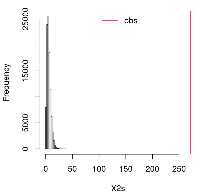
FIGURE 10.5: Empirical sampling distribution of \(X^2\) for an independence test with the assault data.
It is worth remarking that in a test for homogeneity, in the \(r > 2\) case, one can always perform pairwise tests if the null is rejected. That could help narrow down which things are unlike others. As with ANOVA-like methods, be careful with multiple testing hazards (§6.4). Pairwise tests don’t make any sense in an independence context.
10.4 Homework exercises
These exercises help gain experience with \(\chi^2\)-tests for GoF, homogeneity and independence. There are just a couple of math question(s) this time; the rest are coding and/or data analysis. Don’t forget to try each test multiple ways, e.g., via MC or math as appropriate.
Do these problems with your own code, or code from this book. Unless stated explicitly otherwise, avoid use of libraries in your solutions.
#1: Expected \(\chi^2\)
Show (10.4), i.e., that the expected \(\chi^2\) statistic exactly matches the mean of its distribution (10.5), no asymptotics required. Hint: start on the left-hand side, manipulate with linearity of expectations and use facts about multinomial distributions.
#2: Multinomial MLE
Let \(Y \sim \mathrm{Multinom}(n, \theta)\) where \(\theta\) is a \(c\)-vector of probabilities and \(\theta_j > 0\) for all \(j=1,\dots,c\) and \(\sum_{j=1}^c \theta_j\) = 1. Note that this is the same as \(O \sim \mathrm{Multinom}(n, \theta)\) from earlier in the chapter, just re-labeled. Derive the MLE \(\hat{\theta}\).
#3: Two-liner GoF test
Given n and x2, use rmultinom to develop code that furnishes \(N\) MC
samples of \(\chi^2\) GoF statistics (§10.1) with one line,
and calculates a \(p\)-value with a second line.
#4: MC for \(r \times c\) tables via multinomial
Rewrite the MC for homogeneity and independence sampling
(§10.3) so that it avoids sampling data-pairs (via
sample for Cs and Rs followed by table) and instead directly creates
Os via rmultinom. Think of this as an upgrade to the use of rmultinom
for GoF tests (§10.1) for \(1 \times c\) tables to \(r \times
c\) tables. This is not simple even though the code is short.
#5: monty.chisq for all cases
Write a library function that covers all variations of Pearson \(\chi^2\)
tests from the chapter. This includes GoF (§10.1),
homogeneity and independence tests (§10.1) in both MC and
closed-form/asymptotic variations. Use chisq.test to check your work, but
otherwise develop the implementation yourself. Optionally, incorporate your
solutions to #3–4, above.
Hint: many of the following questions are easier after this one is squared away.
#6: Transportation study
Al-Ghamdi (2001) presents a theoretical model for the time elapsed between vehicles on urban roads along with an analysis on observational data collected in Riyadh, the capital city of Saudi Arabia. Those pairs of values, recorded in seconds and categorized into two-second bins, are provided below.
veh <- rbind(
  observed=c(18, 28, 14, 7, 11, 11, 10, 8, 30),
  theory=c(23, 18, 16, 13, 11, 9, 20, 8, 19)
)
colnames(veh) <- c("0-2s", "2-4s", "4-6s", "6-8s", "8-10s", "10-12s",
  "12-18s", "18-22s", ">22s")
What do you think? Does the theoretical model do a good job of explaining those observed values?
#7: Mendelian inheritance
Gregor Mendel’s principles for predicting genetic inheritance experimental tests made validation difficult. One of the earliest applications of Pearson \(\chi^2\)-tests aimed at a quantitative assessment of the theory in real experiments (Harris 1912). That (very old) paper reports many excellent experiments that can be used to test your understanding of GoF tests. Here’s just one. (Note that the author uses the term “calculated” instead of “expected”.)
Crossing a first-generation of pea plants producing yellow, round seeds with pea plants producing green, wrinkled seeds yielded the following observed plants (seeds) in the second generation.
Assuming independent genes, each with a dominant and recessive allele, Mendel’s theory predicts a 9:3:3:1 phenotypic ratio. Do these data support this?
#8: Are 911 calls Poisson?
Data below tally the number of 911 emergency calls within the span of an hour, across 50 randomly chosen hours, in a certain jurisdiction. The default model for such data is Poisson.
y <- c(5, 4, 0, 0, 6, 1, 3, 4, 1, 1, 0, 1, 2, 6, 4, 3, 0, 3, 5, 3, 2,
  8, 6, 1, 4, 3, 1, 3, 1, 1, 0, 3, 5, 4, 1, 9, 0, 5, 1, 1, 1, 12, 0,
  2, 3, 1, 1, 0, 2, 4)
Is it reasonable to use a Poisson to model these data?
Hint: first choose the parameter for the Poisson. Then, table(y) can help
you determine bins for o, however it might be sensible to merge all bins
with just one observation.
#9: Math scores for less affluent students
Revisit the (N)ELS math score data, but this time rather than separating out a particular school, look at all math scores at all schools for students in the bottom half of the socioeconomic spectrum.
## [1] 1021Is it reasonable to study this sample with a Gaussian distribution? Since this is a much larger sample compared to any single school, consider using a larger/finer mandoline (choose larger \(c\)).
#10: ROI with Gaussian?
Refer back to roi$company and roi$industry from §2.5. Recall that these data are available as roi.RData on the book webpage.
Is it reasonable to model either of these samples with Gaussian distributions? In other words, can the P-analyses from the first half of the book be trusted, or should we rely on the non-P ones in the second half? Be careful not to use bins with too few observations.
#11: Women’s health
Assaf et al. (2016) report on a randomized control trial of almost 50,000 women meeting certain criteria (healthy, age 50-79, etc.), exploring relationships between nutrition and long-term health. Data from that study were summarized and cross-referenced against incidence of coronary heart disease (CHD) for treatment (healthy diet) and control populations.
o <- rbind(
  c(1000, 18541),
  c(1549, 27745)
)
colnames(o) <- c("treatment", "control")
rownames(o) <- c("chd.yes", "chd.no")
Is there evidence of a difference in CHD incidence for these two groups?
#12: Math and stat grades
CMDA 2006 is an integrated topics course taught at Virginia Tech (VT), where I work. Most classes at VT are 3 credits, but this one is 6 credits, because it’s basically two classes in one. Although students register once, there are two different professors separately covering math and stats topics, two sets of homeworks, and two sets of midterms. (I have taught the stats half several times, and much of the material from that class went into this book.) There is a combined final, and ultimately students are assigned just one, combined letter grade. However, it is interesting to see what separated grades would be right before the combined final.
Data below record a breakdown of pre-final letter grades on math and stats
halves of CMDA 2006 tallied over several semesters/sections. Category O
combines letter grades D, F, and any other special cases like withdraw and
incomplete.
o <- rbind(
  c(32, 13, 20, 10),
  c(20, 25, 21, 10),
  c(11, 13, 23, 11),
  c(8, 9, 10, 19))
rownames(o) <- c("stats.A", "stats.B", "stats.C", "stats.O")
colnames(o) <- c("math.A", "math.B", "math.C", "math.O")
Is performance on the stats half independent of the math half?
#13: Other assault columns
Revisit analysis of the assault data from §10.3, but
choose two different pairs of columns. For example, look at police with
ER or year with female. Perform an appropriate (homogeneity or
independence) test. Be clear in your explanation of why a particular test
was conducted and what the hypotheses and conclusions are.
#14: Median test
Alright, here is perhaps my biggest indulgence in the book. I’m going to lecture to you in a homework exercise. Bear with me, it’ll be worth it.
The median test is an application of Pearson’s \(\chi^2\)-test where there are “columns”, defined by counts of numbers of samples from populations, arranged in “rows”, indicating above and below the median, respectively.13 Words “columns” and “rows” are in quotes, because actually median test tables are transposed in most presentations. What I mean is, there are actually \(c=2\) rows and \(r\) columns for each of \(r\) populations. I think that’s because a short and fat table looks better on the page than a tall and skinny one.
Let \(y^{(n/2)}\) denote the grand median from all \(n = n_1 + \dots + n_r\) samples. Then, let \(o_{1i}\) count the number of observations from the \(i^\mathrm{th}\) sample that exceed \(y^{(n/2)}\); and let \(o_{2i} = n_i - o_{1i}\) be the number that is less than or equal to that value. See the CT depicted in Table 10.6.
| pop 1 | pop 2 | \(\cdots\) | pop \(r\) | total | |
|---|---|---|---|---|---|
| > \(y^{(n/2)}\) | \(o_{11}\) | \(o_{12}\) | \(\cdots\) | \(o_{1r}\) | \(a = \sum_i o_{1i}\) |
| \(\leq y^{(n/2)}\) | \(o_{12}\) | \(o_{22}\) | \(\cdots\) | \(o_{2r}\) | \(b = \sum_i o_{2i}\) |
| total | \(n_1\) | \(n_2\) | \(\cdots\) | \(n_r\) | \(n = \sum_i n_i\) |
The null hypothesis is that all \(r\) populations have the same median, versus the alternative that at least two have different ones. Test statistic \(x^2\) is the same as usual (10.3); however, when you consider that \(o_{2i} = n_i - o_{1i}\), and that there are only two rows, some simplification arises.
\[ x^2 = \frac{n^2}{ab} \sum_{i=1}^c \frac{\left(o_{1i} - \frac{n_ia}{N} \right)^2}{n_i} \quad \mbox{ and } \quad X^2 \sim \chi^2_{c-1}. \]
As with any other heterogeneity-like test with multiple populations, one can pair them off order to determine which (pairs) are actually different from one another (if the null is rejected). These would be \(2 \times 2\) tables, for which there are specially built methods like Fisher’s exact test.
Ready to give it a try?
Shelf height at supermarkets is important for sales. In a study of sales of breakfast cereal, four shelf heights were varied. The list below records sales in thousands of dollars for cereal brands at those heights.
sales <- list(
    feet=c(8.1, 6.5, 6.6, 8.1, 7.5, 6.7, 9.1, 7.0),
    knee=c(7.9, 8.1, 7.6, 8.1, 8.5, 7.7, 8.5, 7.6, 8.0),
    waist=c(9.0, 8.8, 9.5, 9.4, 9.1, 9.2, 9.5, 8.9),
    eye=c(8.9, 8.8, 8.6, 8.7, 8.2, 8.3, 8.3, 8.8, 9.3))
Do these data indicate that shelf-height affects median cereal sales? Conduct the test via MC and in closed form/asymptotically.
Hint: begin by making Table 10.6 in R.