Chapter 4 A little math: asymptotics

In statistics, asymptotic analysis is the study of properties of an estimator or statistic as the training data size gets large: \(n \rightarrow \infty\). Alas, that’s an unrealistic setting. We never get infinite data. Asymptopia is at once a pipe dream and also irrelevant. The population of women in the United States is finite, so it’s total nonsense to ponder a sample of infinitely many women’s heights.

Nevertheless, contemplating the behavior of estimators or statistics as \(n\) gets large is helpful. You want those quantities to have good properties if and when you can collect more data, and it’s interesting to wonder what happens in the limit as you take that to an infinite extreme. Quantities with good “asymptotic properties”, in the lingo, have another feather in their cap, like unbiasedness or small mean-squared error, connecting back to §3.1. They lead to new statistical procedures and insight. Estimators adjusted to have good asymptotic properties form the basis of many classical statistical tests – in many cases, ones that are easier to perform but also sometimes harder to intuit.

Here I’ll review two key forms of asymptotics. I say “review” because I’m not going to be able to prove everything to you. That’s beyond the scope of the book and, if I’m being honest, my own capabilities. Yet both are beautiful, if a little antique. They’re not – in my not-so-humble opinion – really necessary if you have a computer. Yet they reveal important truths about common procedures and enable you to make calculations mostly by hand, which can be valuable in a pinch, like when your laptop battery dies, and you need a good answer right away.

These two forms of asymptotics are related to one another, and so they often lead to the same place. One is a simple truth about averages (more specifically about sums), and the other about maximum likelihood. MLEs are often sums or averages, so there you go. You may have studied the first one before, and there’s no harm in review. I’m pretty sure the second one will be new to you.

4.1 Central limit theorem

Recall our discussion – a digression really – from §2.1 about the distinction between an average and a mean. They’re not the same thing, but they are related. An average is a quantity that you can calculate from data, whereas a mean is what you expect from averages if you calculate them over and over again. I showed you that an average is unbiased for the mean. Alright, that’s the context we’re working in, generally speaking. Here we go with more specifics. The central limit theorem (CLT) says even more about those averages as they relate to the mean (and to the variance).

Consider \(n\) observations \(y_1, \dots, y_n\). Assume that each \(Y_i\), for \(i=1, \dots, n\), is independent and identically distributed (iid) with mean \(\mu\) and variance \(\sigma^2\), that is, \(\mathbb{E}\{Y_i\} = \mu\) and variance \(\mathbb{V}\mathrm{ar}\{Y_i\} = \sigma^2\). Notice that I’m being very careful here. I’m saying that each \(Y_i\) is independent of the others and comes from the same distribution, and that the moments of that distribution are \(\mu\) and \(\sigma^2\). What’s even more important is what I’m not saying: what the distribution actually is. In particular, I’m not saying it’s Gaussian. It could be Poisson, Bernoulli, gamma, exponential, Pareto, Bobby (once they decide to name a distribution after me), or whatever. It doesn’t matter. In fact, the CLT is most useful when you don’t know the distribution, but it can still be useful even when you do.

The CLT says the following. Let \(\bar{Y}_n = \frac{1}{n} \sum_{i=1}^n Y_n\) denote the average of \(n\) random \(Y_i\) values. Previously I used \(\bar{Y}\) for this without the \(n\) subscript. Here \(n\) matters a lot to the statement of the CLT, so I’m indicating, with my average notation via \(\bar{Y}_n\), how many \(Y_i\)-values are involved.

\[\begin{equation} \bar{Y}_n \sim \mathcal{N}(\mu, \sigma^2/n) \quad \mbox{ as } \quad n \rightarrow \infty. \tag{4.1} \end{equation}\]

Let me help you appreciate, and interpret, this amazing result. No matter what distribution your data come from, the distribution of their average is Gaussian. But they must be iid and you’ve gotta have lots.

You never have infinite \(n\), so the CLT provides approximation for whatever \(n \ll \infty\) you do have, and the approximation is better the bigger \(n\) is. Moreover, you have the same unbiasedness and learning efficiency, via \(\sigma^2 / n\), as you did in the Gaussian case in §2.1. Just interpret things approximately.

Before turning to examples, I want to talk about two variations or special cases. You’ll often see the CLT quoted for sums instead of averages. Just multiply everything by \(n\) and you get \(\sum Y_i \sim \mathcal{N}(n \mu, n\sigma^2)\) as \(n \rightarrow \infty\). I think this version is less useful for statistical inference where averages play a key role, but it does have important applications. A more useful variation involves standardization, like I did for testing with \(z\) statistics in Eq. (3.10).

\[\begin{equation} Z\equiv\frac{\bar{Y}_n - \mu}{\sigma / \sqrt{n}} \sim \mathcal{N}(0, 1) \quad \mbox{ as } \quad n \rightarrow \infty. \tag{4.2} \end{equation}\]

So all averages are standard Gaussian, with pdf \(\phi\) and cdf \(\Phi\), if you center them with their mean \(\mu\) and divide by the standard error \(\sigma/ \sqrt{n}\). This is an approximation, but it’s accurate when \(n\) is large. In some sense, a consequence of this result is that every statistical test based on averages boils down to a \(z\)-test, approximately. To make use of this, you must know, or work out, what \(\mu\) and \(\sigma^2\) are for the distribution you assume generates the data.

Remember, you get to choose the test statistic in Alg. 1.1. If you choose to do it with averages, you can use the CLT. Another consequence of Eq. (4.2) is that quantiles from a Gaussian distribution can be used to form an approximate confidence interval (CI). Eq. (3.19) can be used, and will be exact when \(n \rightarrow \infty\).

How good are these approximations for particular \(n\)? How big should \(n\) be to trust the CLT? Those are, in some sense, the same question. Unfortunately, there’s no simple answer, requiring case-by-case analysis. It’s also too technical for us, and would take up way too much space. Besides, the point is moot. You wouldn’t use a CLT-based \(z\)-test or CI if you could do an exact one, making it an option of last resort. Still, the calculations behind tests in many software libraries utilize the CLT directly, or a CLT-adjacent argument. I’m mostly showing it to you here so that you can take in this awesome fact about averages, and (more importantly) so you understand and can duplicate results that you see from software packages.

Toss up CLT

According to Wikipedia, a Bernoulli distribution with parameter \(\theta\) has mean \(\mu = \mathbb{E}\{Y_i\} = \theta\) and variance \(\sigma^2 = \mathbb{V}\mathrm{ar}\{Y_i\} = \theta (1 - \theta)\). Therefore, our test statistic has the following asymptotic sampling distribution.

\[\begin{equation} \bar{Y}_n \sim \mathcal{N}(\theta, \theta(1 - \theta)/n) \quad \mbox{ as } \quad n \rightarrow \infty \tag{4.3} \end{equation}\]

A standardized version follows Eq. (4.2) similarly.

The trouble with this is that we don’t know \(\theta\), so there’s a chicken or egg problem when it comes to the variance of the sampling distribution. Having \(\theta\) in the mean of the Gaussian is fine. That’s where the quantity of interest, from the null hypothesis, usually is. Things are quirky with a Bernoulli distribution, because it has just one parameter \(\theta\), doing double-duty to determine both location and scale.

Fortunately, our willingness to work in an asymptotic framework helps here. The weak law of large numbers (WLLN) says that

\[\begin{equation} \bar{Y}_n \rightarrow \mu \quad \mbox{ as } \quad n \rightarrow \infty \tag{4.4} \end{equation}\]

Why is this true? The short answer is because of Eq. (4.1). As \(n \rightarrow \infty\) the variance \(\sigma^2/n \rightarrow 0\) and the Gaussian becomes a point spike density centered at \(\mu\). The long answer, supporting theory for laws of large numbers more broadly, is a topic for another text. What does it mean for us? It means we don’t change the asymptotics by slotting in \(\hat{\theta} \equiv \bar{Y}_n\) where \(\theta\) appears in the variance.

In other words

\[\begin{equation} \bar{Y}_n \sim \mathcal{N}(\theta, \bar{Y}_n(1 - \bar{Y}_n)/n) \quad \mbox{ or } \quad \frac{\bar{Y}_n - \theta}{\sqrt{\bar{Y}_n(1-\bar{Y}_n) / n}} \sim \mathcal{N}(0, 1) \quad \mbox{ as } \quad n \rightarrow \infty \tag{4.5} \end{equation}\]

which means we can use a \(z\)-test for \(\theta\) as follows.

se <- sqrt(that*(1 - that)/n)               ## that (=ybar) & n in Ch 1&3 
z <- (that - 0.5)/se                        ## testing H0: theta = 0.5
p.clt <- 2*pnorm(-abs(z)) 
c(clt=p.clt, exact=binom.test(s, n)$p.val)  ## s defined in Chapter 1

##    clt  exact 
## 0.2636 0.3616

These aren’t really that close. What gives? I guess \(n = 30 \ll \infty\), so the approximation isn’t very good. Figure 4.1 provides a comparison of these two sampling distributions, augmenting the view in Figure 3.1. Note the change of variables in the figure that arises from a transformation between \(s_n\) and \(\theta_n\). This is a little advanced, but you don’t really need to worry about it. It’s only really there for the visual.

sgrid <- 0:n
theta <- sgrid/n 
sfun <- stepfun(theta[-1], c(dbinom(sgrid, n, 0.5)))
plot(sfun, xlim=c(0.1, 0.9), xlab="theta", ylab="mass Binom(theta*n, n)", 
  main="", lwd=2)
abline(v=c(that, (n - s)/n), lty=1:2, col=2, lwd=2)
clt <- dnorm(theta, 0.5, sqrt(that*(1 - that)/n))/n  ## change of variables
lines(theta, clt, col=3, lty=3, lwd=2)   
legend("topleft", c("that", "reflect", "clt"), lty=1:3, col=c(2,2,3), 
  lwd=2, bty="n")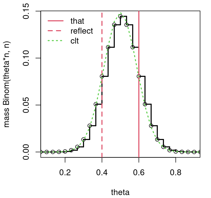

FIGURE 4.1: Extending Figure 3.1 to include a CLT-approximating sampling distribution. The factor 1/n in the clt calculation arises from a transformation between s and theta.

That difference, between discrete and continuous, comprises at least some of the approximation error, which can be visualized in the figure as a gap between dotted green and solid black lines. The Gaussian CLT overestimates on the left, and under on the right. It is clear, however, that larger \(n\), providing more steps in the discrete distribution, provides greater accuracy.

Completing the example, an approximate CI may be calculated as follows.

q <- qnorm(0.975)
CI.clt <- that + c(-1, 1)*q*se
rbind(clt=CI.clt, exact=binom.test(s, n)$conf.int)

##         [,1]   [,2]
## clt   0.4247 0.7753
## exact 0.4060 0.7734

Again, recall from §3.3 that the CI from binom.test is special because it has guardrails to cope with certain edge cases. Nevertheless, those CIs are in close agreement. This asymptotic CI goes by a special name, the Wald interval, and has known drawbacks, although those are not exhibited in this example. I’ll let you read more on that Wikipedia page.

One correction that targets a degenerate case discussed in §3.3, when there are no “heads” and \(\bar{y}_n = 0\) (or no “tails” and \(\bar{y}_n = 1\)), is known as an adjusted Wald interval (Agresti and Coull 1998). At level \(\alpha\) and using \(q_{1-\alpha/2} = \Phi^{-1}(1-\alpha/2)\), an adjusted Wald interval can be interpreted as an interval formed from \(n\) data values plus four “hallucinated” \(y\)-values that contain two heads and two tails:

\[\begin{equation} \tilde{\theta}_n \pm q_{1-\alpha/2} \sqrt{\tilde{\theta}_n(1-\tilde{\theta}_n) / n} \quad \mbox{ where } \quad \tilde{\theta}_n = \frac{n}{n + 4} \bar{y}_n + \frac{4}{n+4} \frac{1}{2}. \tag{4.6} \end{equation}\]

Adding those extra four flips doesn’t change anything asymptotically. As \(n \rightarrow \infty\) we have that \(\tilde{\theta}_n \rightarrow \bar{y}_n\), so an adjusted Wald CI is the same as the Wald one, which converges to the exact interval under the CLT. Note that there isn’t an \(n + 4\) in the denominator of the standard error because those “hallucinated” flips don’t have real information in them, so you wouldn’t want them to reduce the uncertainty or the size of the interval for fixed \(n \ll \infty\).

ttilde <- (n/(n + 4))*that + (4/(n + 4))*0.5
setilde <- se <- sqrt(ttilde*(1 - ttilde)/n)
CI.awald <- ttilde + c(-1, 1)*q*setilde
CI.awald

## [1] 0.4121 0.7643

Having “imagined” flips helps guard against a degenerate \([0,0]\) interval, but does not provide the same correction as the R library, due to Clopper and Pearson (1934).

ttilde <- (6/(6 + 4))*0 + (4/(6 + 4))*0.5
setilde <- se <- sqrt(ttilde*(1 - ttilde)/6)
CI.awald <- ttilde + c(-1, 1)*q*setilde
rbind(awald=CI.awald, clopper=binom.test(0, 6)$conf.int)

##            [,1]   [,2]
## awald   -0.1201 0.5201
## clopper  0.0000 0.4593

It’s unsatisfying to get a CI for \(\theta\), a proportion in \([0,1]\), that includes negative numbers. This is happening because \(n=6\) is very small compared to infinity. In such cases, a CLT approximation can be poor. However, if you report a version of the interval truncated to lie inside \([0,1]\), you get a conservative approximation that is much better than reporting \([0,0]\).

if(CI.awald[1] < 0) { CI.awald[1] <- 0 }
if(CI.awald[2] > 1) { CI.awald[2] <- 1 }
CI.awald

## [1] 0.0000 0.5201

My preference would be to lean the Monte Carlo (MC) interval from §3.3, since I can control the accuracy. However, it could be sensible to borrow the adjusted \(\tilde{\theta}_n\) estimator with its imaginary four flips. I’ve left exploring that to you as a homework exercise.

Location CLT

Maybe I could have skipped this example, but I wanted to continue the flow. It’s nice to have two running examples. Their utility will soon run thin, but first I’d like to squeeze everything out.

When data are modeled as iid Gaussian, \(Y_i \stackrel{\mathrm{iid}}{\sim} \mathcal{N}(\mu, \sigma^2)\), we already know the sampling distribution. The one quoted by the CLT (4.1) is exact for any \(n\), no asymptotics required. See Eq. (3.9) and more broadly §3.2. I showed you how the Gaussian becomes a Student-\(t\) when estimating \(\sigma^2\), resulting in the infamous \(t\)-test and associated intervals (§3.3). Nothing new to add here.

But since I’ve got you, it’s worth additionally remarking on one thing. The CLT is letting us know that, if \(n\) is large, we can approximate a \(t\)-test and CI with a \(z\)-analog. A similar WLLN argument gives that \(\hat{\sigma}_n \rightarrow \sigma\) as \(n\rightarrow \infty\), and likewise for \(s_n\). See Eqs. (3.5) and (3.6), respectively. Therefore, \(\bar{Y}_n \sim \mathcal{N}(\mu, \hat{\sigma}^2/n)\) as \(n \rightarrow \infty\).

Back in the day, Student-\(t\) tables only had quantiles for a limited selection of \(\nu\)-values. There would be some sort of note to use the Gaussian ones for larger \(\nu\). Recall that \(\nu = n - 1\) for our location example. A CLT argument justifies that guidance. These days we can use pt and qt, like in R. So what I’m telling you is largely trivia.

As a practical matter, most folks don’t bother with a Student-\(t\) when \(\nu > 30\). (They often don’t bother with \(z\) tables either, using the \(|z| > 2\) rule to reject.) A rule of thumb of \(n > 30\) is applied a lot more widely (i.e., beyond Gaussian modeling) by appealing to similar logic, regardless of the modeling distribution. Figure 4.1 looks pretty good for the Binomial, and in homework exercises in §4.4 you’ll have a chance to look at some other examples.

4.2 Distribution of the MLE

The statistic you use with a hippopotamus is totally up to you. If you choose a sum or an average, then the CLT is your go-to, that is, assuming you don’t have a computer handy or your mathematical chops don’t lead you to a closed-form sampling distribution. Here I’ll show you that if you limit yourself to MLEs, then you get a double automation benefit. The first is that with an MLE you know that you’re estimating quantities optimally, in a sense. The second is this nice theorem, which I see as an extension of the CLT.

Let \(\theta\) be a \(p\)-dimensional parameter to a family of distributions emitting log-likelihood \(\ell(\cdot)\), and let \(y_1, \dots, y_n\) be modeled as iid from that family. Notice how I’m being coy here not to mention the actual distribution. Like the CLT, the beauty of this result lies in its general applicability. Within reason, and with the details being a bit of a distraction, it doesn’t matter what the distribution is. What matters is the log-likelihood and iid assumption.

Let \(\hat{\theta}_n\) be the \(p\)-dimensional vector maximizing \(\ell(\theta; y_1, \dots, y_n)\). You would find \(\hat{\theta}_n\) by following the procedure outlined in Alg. 3.1, which involves taking partial derivatives. These are the likelihood equations:

\[ \frac{\partial \ell}{\partial \theta_j} \Big{|}_{\hat{\theta}_n} = 0, \quad \mbox{ for } \quad j=1,\dots, p. \]

Then, under some technical conditions, that would (again) be a distraction,

\[\begin{equation} \hat{\theta}_n \sim \mathcal{N}_p \left(\theta, \frac{1}{n} i_1^{-1}(\theta) \right) \quad \mbox{ as } \quad n \rightarrow \infty. \tag{4.7} \end{equation}\]

Above, \(\mathcal{N}_p\) is a \(p\)-variate multivariate normal distribution (MVN), which is a vectorized extension of an ordinary Gaussian distribution. This concept is a little bit of a stretch for this book, but bear with me. Whereas a Gaussian is parameterized by its mean and variance, both scalars, an MVN is parameterized by a mean vector (\(\mu = \theta\) above) and covariance matrix (\(\Sigma = \frac{1}{n} i_1^{-1}(\theta)\)). Notice that since the mean of the distribution for \(\hat{\theta}_n\) is \(\theta\), this means that the MLE is asymptotically unbiased for the true, unknown parameter. Cool, right?

Quick digression for two notes on notation before explaining that \(i_1\) thing. Many authors use a bold font for matrices and vectors, but I’m not going to do that here because we won’t really need it. I’m only making a brief foray into vectorized probabilities. Don’t panic. The main reason to introduce them here is to give you an impression of the bigness, and generality, of the result.

For now, just appreciate that Eq. (3.1) is similar to the CLT (4.1), but better, because it applies to any MLE and for all of its \(p\) parameters! The mean of the MVN is the true, but unknown parameter (i.e., \(\hat{\theta}_n\) is asymptotically unbiased), and the covariance has an \(n\) in the denominator which means that you learn, having lower uncertainty, with more data. I’ll say more about that in a moment.

My second note involves \(\theta\), which is pulling double duty as the true, unknown value that generated the data and as the free variable we differentiate with respect to in order to estimate \(\hat{\theta}_n\). I hope you’ll forgive me that transgression so that we can have things a little more streamlined by not introducing new quantities to keep track of. I’m betting you didn’t notice until I said something, and you possibly still don’t. This is mostly a disclaimer for my more pedantically minded colleagues.

Alright, back to that funny \(i_1^{-1}(\theta)\). The (co-) variance of the derivative of the log-likelihood \(\ell(\theta; Y_1, \dots, Y_n)\) is known as Fisher information (FI). Sometimes you’ll hear it described as the variance of the score. It turns out you can calculate this covariance via the Hessian. Writing \(Y \equiv Y_1, \dots, Y_n\) as a shorthand …

\[\begin{equation} i(\theta) = \mathbb{C}\mathrm{ov} \{\nabla \ell(\theta; Y)\} = - \mathbb{E} \{\nabla \nabla^\top \ell(\theta, Y) \}. \tag{4.8} \end{equation}\]

It’s not too hard to show this is true, but I’d rather spend time pondering its meaning.

The Hessian is a vectorized second derivative (second gradient). First derivatives tell you about slope, and second derivatives about curvature. So FI is expected curvature. Curvature tells you something about how “peaky” the function – in this case the likelihood – is. Peakiness and (co-) variance are one and the same thing, conceptually. For example, the smaller \(\sigma^2\) for a Gaussian, the more peaked the bell curve. The more information you get from the data, measured by FI, the lower your uncertainty. So there should be an inverse relationship between FI and (co-) variance (4.8).

The most important thing about Eq. (4.8) is it explains how to calculate the variance of Gaussian approximation (4.7). An outer product of \((p \times 1)\)-vectors (\(\nabla \nabla^\top\)) gives you a \(p \times p\) matrix. You’ve already taken first derivatives when solving the likelihood equations. Just do it one more time. Here is another fact that helps, allowing me to complete Eq. (4.8). When data are iid, \(\ell(\theta; y_1, \dots, y_n) = \sum_{i=1}^n \ell(\theta; y_i)\). This is a logarithm turning products, via independence, into sums. In that case \(i(\theta) = i_n(\theta) = n i_1 (\theta)\) where \(i_1\) is the FI of a single observation. Said another way, FI from one observation (e.g., \(Y_1\)) can be used to determine FI from all \(n\) observations. You don’t have to hassle with any sums when taking second partial derivatives. That makes the bookwork a lot easier.

Examples are coming momentarily. But first, I want to put it all down procedurally in an Algorithm, augmenting Alg. 3.1 for the MLE. These are steps you would always do after finding \(\hat{\theta}_n\).

Algorithm 4.1: Asymptotic Distribution of the MLE

Assume Steps 1–4 of Alg. 3.1 have already been carried out.

Then

7. Simplify to a one-sample version of the (partial) derivative of the log-likelihood \(\nabla \ell_1 \equiv \nabla \ell(\theta; y_1)\).

\[ \nabla \ell_1 = \left(\frac{\partial\ell_1}{\partial \theta_1}, \dots, \frac{\partial\ell_1}{\partial \theta_p}\right) \]

8. Differentiate again with respect to all \(p\)-components, forming a Hessian.

\[ \nabla \nabla^\top \ell_1 = \left( \begin{array}{ccc} \frac{\partial^2 \ell_1}{\partial \theta_1 \partial \theta_1} & \cdots & \frac{\partial^2 \ell_1}{\partial \theta_1 \partial \theta_p} \\ \vdots & \ddots & \vdots \\ \frac{\partial^2 \ell_1}{\partial \theta_p \partial \theta_1} & \cdots & \frac{\partial^2 \ell_1}{\partial \theta_p \partial \theta_p} \end{array} \right) \]

9. Interpret \(\nabla \nabla^\top \ell_1 \equiv \nabla \nabla^\top \ell (\theta; y_1)\) as a random quantity by replacing \(y_1\) with \(Y_1\) and take its expectation with respect to the distribution of \(Y_1\):

\[ i_1(\theta) = - \mathbb{E} \{\nabla \nabla^\top \ell (\theta; Y_1)\}. \]

Return the asymptotic sampling distribution (4.7).

A few notes. The “Assume” part specifies Steps 1–4 of Alg. 3.1 because those are all that’s required here. Presumably you also did Steps 5–6 calculate the MLE \(\hat{\theta}_n \equiv \hat{\theta}\). You’ll need that too, eventually. Step 7 involves inspecting the form of \(\Delta \ell\) from Step 4 and dropping the sum, replacing \(y_i\) with \(y \equiv y_1\). Step 8 is technically an integral, however, log-likelihoods are often a sum of different quantities involving \(y\), which means you can just replace \(y\)-values (or \(Y\)-values) with \(\mathbb{E}\{Y\}\) by linearity of expectations. Step 10, which in generality would involve a matrix inverse, is just a reciprocal when \(\theta\) is a \(p=1\) scalar, or when the \(p \times p\) matrix \(i_1(\theta)\) is diagonal.

Toss up asymptotic MLE

Eq. (3.2) provides an expression for the derivative of the log-likelihood. Reexpressing that quantity for a single observation \(y_1\) serves as a jumping off point for Steps 7–9 in Alg. 4.1. There are some simplifications here since parameter \(\theta\) is \(p=1\) dimensional. All gradients are scalar derivatives, and so the Hessian is scalar too.

\[ \begin{aligned} & \mbox{7: one-sample derivative} & \ell_1'(\theta; y_1) &= \frac{y_1}{\theta} - \frac{1 - y_1}{1 - \theta} \\ & \mbox{8: second derivative} & \ell_1''(\theta; y_1) &= - \frac{y_1}{\theta^2} - \frac{1 - y_1}{(1 - \theta)^2} \\ & \mbox{9: expectation } & - \mathbb{E}\{\ell''(\theta, Y_1)\} &= \frac{\mathbb{E}\{Y_1\}}{\theta^2} + \frac{1 - \mathbb{E}\{Y_1\}}{(1 - \theta)^2} \\ &&&= \frac{\theta}{\theta^2} + \frac{1 - \theta}{(1 - \theta)^2} \\ && \mbox{so } \quad i_1(\theta) &= \frac{1}{\theta(1-\theta)} \end{aligned} \]

Connecting back to Eq. (4.7), the sampling distribution is therefore

\[ \hat{\theta} \sim \mathcal{N}(\theta, \theta(1 - \theta)/n) \quad \mbox{ as } \quad n \rightarrow \infty. \]

This the same as Eq. (4.3) since \(\hat{\theta} = \bar{Y}_n\). So the CLT and the asymptotic distribution of the MLE are the same, in this Bernoulli case. This happens because \(\hat{\theta}_n = \bar{Y}_n\): same estimator or test statistic, same result for the asymptotic distribution.

One nice thing about the calculations above is that they’re programmatic. Alg. 4.1 tells you exactly what to do. Notice how the two methods use similar, but not identical, information. For the CLT, you have to remember the mean and variance of Bernoulli random variables. (Not a big leap if you’re using a computer connected to the internet.) To calculate the asymptotic distribution of the MLE, you must recall the Bernoulli likelihood, mean and some calculus. (Differentiation is a good transferable skill. Keep it fresh!)

It’s nice when two disparate ideas lead to similar, or identical, conclusions. The same WLLN result (4.4) applies here, replacing \(\theta\) with \(\hat{\theta}\) for variance terms in order to test hypotheses (4.5) and construct CIs (4.6). It also means there’s nothing more for me to do for this example, because I did it all already in §4.1.

Location asymptotic MLE

Continuing on from Eqs. (3.3) and (3.4), and working on both parameters \(\mu\) and \(\sigma^2\) simultaneously, we have …

\[ \begin{aligned} & \mbox{7: one-sample derivative} & \frac{\partial \ell_1}{\partial \mu} &= \frac{y_1 - \mu}{\sigma^2} & \mbox{and} && \frac{\partial \ell_1}{\partial \sigma^2} &= - \frac{1}{2\sigma^2} + \frac{(y_1 - \mu)^2}{2(\sigma^2)^2} \\ & \mbox{8: second derivative} & \frac{\partial^2 \ell_1}{\partial \mu^2} &= - \frac{1}{\sigma^2} & \mbox{and} && \frac{\partial^2 \ell_1}{\partial (\sigma^2)^2} &= \frac{1}{2(\sigma^2)^2} - \frac{(y_1-\mu)^2}{(\sigma^2)^3} \\ && \frac{\partial^2 \ell_1}{\partial \mu \partial \sigma^2} &= - \frac{y_1-\mu}{(\sigma^2)^2} \end{aligned} \]

Next, collect everything in a matrix, using \(\frac{\partial^2 \ell_1}{\partial \mu \partial \sigma^2} = \frac{\partial^2 \ell_1}{\partial \sigma^2 \partial \mu}\), and take expectations.

\[ \begin{aligned} & \mbox{9: expectation } & - \mathbb{E} \{\nabla \nabla^\top \ell(\theta, Y_1)\} &= \left[ \begin{array}{cc} \frac{1}{\sigma^2} & \frac{\mathbb{E}\{Y_1\} - \mu}{(\sigma^2)^2} \\ \frac{\mathbb{E}\{Y_1\} - \mu}{(\sigma^2)^2} & -\frac{1}{2(\sigma^2)^2} + \frac{\mathbb{E}\{(Y_1 - \mu)^2\}}{(\sigma^2)^3} \end{array} \right] \\ && \mbox{so } \quad i_1(\theta) &= \left[ \begin{array}{cc} \frac{1}{\sigma^2} & 0 \\ 0 & \frac{1}{2(\sigma^2)^2} \end{array} \right] \end{aligned} \]

The last line, above, follows since \(\mathbb{E}\{Y_1\} = \mu\) and \(\mathbb{E}\{(Y_1 - \mu)^2\} = \mathbb{V}{\mathrm{ar}}\{Y_1\} = \sigma^2\).

So what does this mean when plugging into Eq. (4.7)? Did we learn anything? The FI matrix is diagonal, and so then too is its inverse. This means that the components of \(\hat{\theta} = (\hat{\mu}, \sigma^2)\) are uncorrelated with one another, and under a Gaussian means they’re statistically independent. So they may be studied in isolation.

Looking just at the first component, we have \(\hat{\mu} \sim \mathcal{N}(\mu, \sigma^2/n)\), as \(n \rightarrow \infty\). We already knew that result was exact for any \(n\); no asymptotics required. Looking at the second component,

\[\begin{equation} \hat{\sigma}^2 \sim \mathcal{N}(\sigma^2, 2\sigma^4/n) \quad \mbox{ as } \quad n \rightarrow \infty. \tag{4.9} \end{equation}\]

If we didn’t know anything about \(\chi^2_\nu\) distributions, that could serve as an approximation. I didn’t do this particular case in §3.2, focusing instead on \(s^2\) in Eq. (3.16), but a similar calculation provides \(\hat{\sigma}^2 \sim \frac{\sigma^2}n \chi^2_n\). Figure 4.2 offers a comparison of actual and approximate distributions for the – somewhat arbitrarily chosen – case of \(n=20\) and \(\sigma^2=1\).

sigma2 <- 1
n <- 20
s2grid <- seq(0, 3, length=1000)
plot(s2grid, dchisq(s2grid*n, n)*n/sigma2, ## from change of variables
  type="l", lwd=2, ylab="density", xlab="s2hat")
lines(s2grid, dnorm(s2grid, sigma2, sqrt(2/n)), col=2, lty=2, lwd=2)
legend("topright", c("actual", "approx"), lty=1:2, col=1:2, lwd=2, bty="n")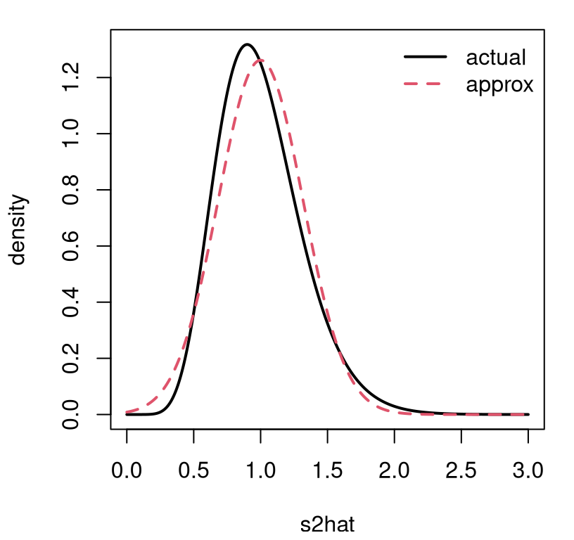

FIGURE 4.2: Comparing a Gaussian asymptotic approximation of the distribution of \(\hat{\sigma}^2\) to the actual \(\chi^2_n\) for \(n=20\) and \(\sigma^2 = 1\). Factor n/sigma2 in dchisq arises from a change of variables, scaling \(\chi^2_n\) deviates by \(n/\sigma^2\).

Observe that the approximation is good, but not perfect. It would improve for larger \(n\). I encourage you to try other \(\sigma^2\) and \(n\) values.

---

I’ve shown you two examples of how a Gaussian, which is a distribution for real-valued random variables (both positive and negative), can approximate the distribution of two very different estimators. For coin tosses, it can approximate a discrete, binomial sampling distribution, where the estimator is a natural number (non-negative integer) because it is a sum of binary flips. For location data, it can approximate the distribution of a positive, variance quantity with a \(\chi^2_\nu\) distribution. If you’re a nerd like me, you’ll think that’s pretty neat.

I want to make a final remark here on efficiency, mirroring a discussion from §2.2 where we studied uncertainty in estimators as a function of training data size, \(n\). The Cramer-Rao lower bound (CRLB) says that, under certain technical conditions that I won’t bore you with, the variance of an unbiased estimator \(\hat{\theta}_n\) of \(\theta\) can be no smaller than the (squared) standard error of the asymptotic (Gaussian) sampling distribution of the MLE.

That is, \[ \mathbb{V}\mathrm{ar}\{\hat{\theta}_n\} \geq \frac{1}{n} i_1^{-1}(\theta). \]

This is really cool! The CRLB says that the Gaussian sampling distribution (4.7) is efficient, at least asymptotically. It says you can do no better than \(\frac{1}{n} i_1^{-1}(\theta)\), when it comes to uncertainty about \(\hat{\theta}_n\), and Eq. (4.7) achieves that variance. Using the MLE gives you the optimal rate of learning for unbiased estimators, in a certain sense.

4.3 Asymptopia and Monte Carlo

There’s an important distinction to make about asymptopia. Remember how I said in §1.3 that you get a better approximation with MC as \(N \rightarrow \infty\). Here, with the CLT or asymptotic distribution of the MLE, I’m telling you that you get a better approximation with a Gaussian as \(n \rightarrow \infty\). Both infinities are out of reach, past the end of the universe, but that doesn’t mean they’re the same thing.

We have control over computational effort, \(N\), in a MC simulation. So long as we’re willing to wait a little longer, we can get a better approximation with bigger \(N\). As statistical analysts, we almost never have control over \(n\). The experiment has been performed, or the survey has been gathered, and no more data (bigger \(n\)) is coming any time soon. We’re stuck with what we’ve got.

The CLT and approximate distribution of the MLE are beautiful results. For a long time they were very important, practical results. They saved a lot of hassle. For many tests, all you need is a \(z\)-table, and you’re good to go. But times have changed. Lookup tables are out and computing is in. MC is intuitive, highly accurate (for large \(N\)), and as time goes on, will become even more powerful and easy to use. Computer hardware and software are getting better all the time.

Going forward, I’ll do my best to navigate concepts with MC, while grounding outcomes by drawing comparisons to library output. Sometimes those libraries utilize exact, closed-form calculations. Other times they leverage asymptotics. I’ll try to send a clear signal about which is which. When libraries leverage asymptotic results, it’ll be hard to make a precise quantitative comparison to a MC alternative because both are approximations. However, I shall encourage you to draw comfort from the fact that MC can always be made to be more accurate with larger \(N\). In my mind, that casts doubt on the precision of a calculation based on asymptotics. But that’s only my opinion.

Taking things to extremes (\(n \rightarrow \infty\)) is a fine way to study a mathematical procedure, or to stress test an engineered system. Yet real decisions with real consequences are made from finite, and often limited information. When data are few (small \(n\)), statistical thinking and methodology shine the most. If it’s done right.

4.4 Homework exercises

These exercises are more analytical than those in other chapters, although there’s still some coding to do. Most questions involve revisiting exercises from §3.5 using the CLT or asymptotic distribution of the MLE.

At the risk of being too repetitive, use methods from this chapter, not previous chapters or other materials. Deploying non-Chapter 4 methods here will likely not earn full credit. Do these problems with your own code, or code from this book. I encourage you to check your work with library functions. However, check with your instructor first to see what’s allowed. Unless stated explicitly otherwise, avoid use of libraries in your solutions.

#1: Poisson

Revisit exercise #1 from §3.5.

1. Approximate the sampling distribution for \(\hat{\theta}_n\) using the CLT.
2. Now do it using the asymptotic distribution of the MLE.
3. Using data values provided in §3.5 #1, test the hypothesis in #1c using your results from parts #a and #b above.
4. Provide a 95% CI using your results from parts #a and #b above.

#2: Exponential

Revisit exercise #2 from §3.5.

1. Why might it be difficult to approximate the sampling distribution for \(\hat{\theta}_n\) using the CLT? (It’s not impossible, but I would treat this as a challenge problem and move on to #b.)
2. Approximate the sampling distribution for \(\hat{\theta}_n\) using the asymptotic distribution of the MLE.
3. Using data values provided in §3.5 #2, test the hypothesis in #1c using your results from part #b above.
4. Provide a 95% CI using your results from part #b above.

#3: Scale-1 Pareto

Revisit exercise #3 from §3.5.

1. Why might it be difficult to approximate the sampling distribution for \(\hat{\theta}_n\) using the CLT? (It’s not impossible, but I would treat this as a challenge problem and move on to #b.)
2. Approximate the sampling distribution for \(\hat{\theta}_n\) using the asymptotic distribution of the MLE.
3. Using data values provided in §3.5 #3, test the hypothesis in #1c using your results from part #b above.
4. Provide a 95% CI using your results from part #b above.

#4: Update monty.bern with asymptotic calculations

Update monty.bern from §1.4, and possibly also §3.5 #6, to include approximate Gaussian testing and CI calculations from this chapter, including optional visuals. Follow these specifications.

• Provide both ordinary and Wald CIs if the data have at least one head and one tail.
• Otherwise, provide an adjusted Wald interval, and be sure to note which interval is provided with your output.
• Update your MC CI implementation to use a modified \(\hat{\theta}_n\) from the adjusted Wald interval in the case where the sample does not contain at least one head or tail.
• Check N, and if N == -1 use an asymptotic approximation instead of MC or exact calculations. That way the same library function can be used for any of the methods you’ve learned so far.
• Test this new capability by checking that results are similar to those you got on earlier homeworks. (Careful, they won’t be identical.)

#5: Revisit Bernoulli

Revisit any of Exercises #2 (silicone wafers), #3 (PVC or copper piping), or #4 (GPS speed vs. speedometer) from §1.5, but do it with an asymptotic approximation, including CIs. (This will be pretty easy if you already did #4 above.)

#6: Explore Wald adjustments

Study the adjusted Wald CI, and contrast it to the Clopper and Pearson (1934) interval provided by binom.test in R, when the observed data has all \(n\) heads, and no tails, for \(n=2, \dots, 100\). Plot the upper and lower bounds for both intervals, on the same axes, as a function of \(n\). That’s four lines on one plot (use color/line types). (This is easier if you’ve already done #4 above.)

References

Agresti, A., and B. A. Coull. 1998. “Approximate Is Better Than ‘Exact’ for Interval Estimation of Binomial Proportions.” The American Statistician 52 (2): 119–26.

Clopper, C. J., and E. S. Pearson. 1934. “The Use of Confidence or Fiducial Limits Illustrated in the Case of the Binomial.” Biometrika 26: 404–13.