Chapter 11 Non-P scale
Scale is to variance as location is to mean. This chapter is the non-P version of Chapter 6’s P. It’s not common to test variance nonparametrically for just one sample. If that’s what you’re looking for – a non-P version of §6.1 – there’s always the bootstrap (Chapter 8).
Previous chapters covered concepts in pairs, and this one is no different. Here I cover the so-called squared ranks test and Kruskal–Wallis test. Squared ranks targets a comparison of scale, or spread, of samples from two populations – a non-P §6.2. Kruskal–Wallis is like non-P ANOVA. That’s an unofficial designation but, like ordinary/P ANOVA (§6.3), juxtaposing residual scales allows locations to be compared across multiple samples.
11.1 Squared ranks
Consider a two-sample setup with \(y_1, \dots, y_{n_y}\) and \(x_1, \dots, x_{n_x}\) being mutually independent but possibly not from the same distribution. Mutually independent is a fancy way of saying that samples are independent from one another, and also (at least in this case) that they’re iid within-sample. Interest lies in testing if these samples come from the same distribution, \(F_Y = F_X\), i.e., that they are iid across both samples. Competing hippopotami are just like in Eq. (9.2), but with \(\mathbb{E}\) swapped for \(\mathbb{V}\mathrm{ar}\). In other words, focus here is on variance.
\[\begin{align} \mathcal{H}_0 &: \mathbb{V}\mathrm{ar}\{Y\} = \mathbb{V}\mathrm{ar}\{X\} && \mbox{null hypothesis (“what if")} \tag{11.1} \\ \mathcal{H}_1 &: \mathbb{V}\mathrm{ar}\{Y\} \ne \mathbb{V}\mathrm{ar}\{X\} && \mbox{alternative hypothesis} \notag \end{align}\]
Writing things out with variances rather than expectations clarifies the mindset, but ultimately if distributions are the same then any aspect is the same. What matters is how a chosen statistic provides a wedge that, under the null hypothesis, reveals a clear probabilistic contradiction in favor of an alternative. Whenever \(\mathbb{V}\mathrm{ar}\{Y\} \ne \mathbb{V}\mathrm{ar}\{X\}\) that implies \(F_Y \ne F_X\), and sometimes you’ll see alternative hypotheses written out that way instead. The preferred statistic involves a study of how far individual data points are from their averages. This isn’t exactly “variance”, but it’s closely related. Hence hedging the name of the chapter with “scale”.
Convert each \(y_i\) and \(x_j\) into its absolute deviation from its corresponding sample average. That is, let
\[ \begin{aligned} v_i &= |y_i - \bar{y}| & \mbox{for } \quad i&=1, \dots, n_y \\ \mbox{and } \quad u_j &= |x_j - \bar{x}| & \mbox{for } \quad j&=1, \dots, n_x. \end{aligned} \]
Assign ranks (§9.1) to the combined sample \(v_1,\dots,v_{n_y},u_1,\dots,u_{n_x}\) using average ranks when there are ties. Let \(r_1^{(v)},\dots,r_{n_y}^{(v)}\) and \(r_1^{(u)},\dots, r_{n_x}^{(u)}\) denote those ranks. As with other tests based on ranks there are several common test statistics, and I’ll show you a couple of them.
First comes the eponymous squared ranks, which are the squared analog of \(\bar{r}\) from a Wilcoxon rank sum test (9.3).
\[\begin{equation} \bar{r}^2 \equiv \bar{r}^{2(v)} = \sum_{i=1}^{n_y} r_i^{2(v)} \tag{11.2} \end{equation}\]
In words, \(\bar{r}^2\) is the sum of squared ranks corresponding to \(v\), which are absolute deviations for \(y\). Ranks for \(u\), via \(x\), are not directly involved, but instead occupy the “negative space”. It would be equivalent to using a sum of squared \(u\) ranks, being diligent to keep everything else straight downstream. It doesn’t matter which sample is labeled with \(x\) and which with \(y\). Careful here not to get \(\bar{r}^2\) confused with \(r^2\) which is a squared correlation from §7.2. It’s unfortunate that both rank, and sample correlation use the letter \(r\).
Following logic similar to Eq. (9.4), we may deduce that
\[\begin{equation} \mathbb{E}\{\bar{R}^2\} = \frac{n_y(n + 1)(2n + 1)}{6} \quad \mbox{ under } \mathcal{H}_0, \tag{11.3} \end{equation}\]
because Eq. (11.2) is tallying \(n_y\) (random) parts of a square pyramidal number. You don’t have to take my word for it. I’ll show how that theoretical expectation compares to a MC one momentarily.
That’s pretty much it. Before turning to strategies for assessing the sampling distribution of \(\bar{r}^2\), I shall pause to introduce a running example. I hope that will help clarify details of the development so far in code. In keeping with themes from Chapter 9, consider a study tallying the numbers of bicycles on Metro train lines. Data below record counts of bikes observed on Green- (\(y\)) and Orange-line (\(x\)) trains during randomly chosen commute hours.
y <- c(46, 51, 61, 70, 66, 69, 50, 44, 58, 59, 49, 54)
x <- c(74, 72, 90, 51, 65, 63, 100, 57, 82)
ny <- length(y)
nx <- length(x)
Here are the relevant calculations in R. First, form absolute deviations from sample averages.
Then form the combined ranking.
Extract the part of the ranking due to v (or y) and calculate the test
statistic (11.2).
## [1] 1390As in Chapter 9, it’s worth knowing whether or not there are ties in the ranks, since that might affect strategies for determining the sampling distribution.
## [1] 0No ties, so there’s nothing to worry about. In Chapter 9 I had two running examples, one with ties and one without. I did that twice over, for Wilcoxon and signed rank tests, respectively. Things got complicated to keep track of, code wise, and in the end there wasn’t much value added except a takeaway that concerns may be overblown. Here, I shall keep it simple with one example, and provide pointers to possible audibles in the presence of ties.
Squared ranks test by MC
Much can be borrowed from the Monte Carlo (MC) for Wilcoxon rank sum tests.
Since there are no ties, no special extensions to virtualize random ties in
ranks are required. If you do encounter ties, and wish to entertain those,
rank.ties in rank_ties.R on
the book webpage is equally applicable here. Really, the only difference
compared to Wilcoxon tests is how the statistic is calculated in the last line
of the loop.
N <- 1000000
n <- length(r)
R2bars <- rep(NA, N)
for(i in 1:N) {
  Rvus <- sample(1:n, n)
  Rvs <- Rvus[1:ny]
  R2bars[i] <- sum(Rvs^2)
}
According to Eq. (11.3), the mean of this distribution may be calculated as follows.
## [1] 1892 1892Identical, though that’s not guaranteed. Either (if they are different) may
be used to reflect an observed statistic for visualization purposes. I shall
skip that here and go straight to the \(p\)-value, but R2mean will come back
later. For now, note that r2bar is less than R2mean, so the tail
calculation is on the left side.
## [1] 0.1188There’s not enough evidence to reject \(\mathcal{H}_0\). For now, it seems that the number of bikes on Green- and Orange-line trains come from the same distribution, at least as regards their scale.
Squared ranks test by math
As with Wilcoxon tests, you can turn evaluation of the mass function of the test statistic under the null into a subset sum problem (SSP). Since ranks are being squared, yielding bigger sums, we have a harder SSP as compared to ordinary ranks. Why? Many more combinations could be formed to reach those larger sums.
Details are left to §B.3. Here I shall just take dsqranks
and psqranks from ranks.R on the book
webpage, providing mass and cumulative distribution, respectively.
Figure 11.1 shows what you get for Metro bikes. Go ahead and peek at it – what a strange distribution! Consecutive integers can have wildly different numbers of ways that squares can sum into them, and thus wildly different masses.
r2grid <- 500:3000
dr2 <- rep(NA, length(r2grid))
denom <- dsqranks.denom(ny, nx)  ## faster with denom pre-calculated
for(k in 1:length(r2grid))
  dr2[k] <- dsqranks(r2grid[k], ny, nx, denom=denom)  ## used here
plot(r2grid, dr2, type="l", lwd=2,
  xlab="r2bar", ylab="mass dsqranks(r2bar, ny, nx)")
abline(v=c(r2bar, 2*R2mean - r2bar), col=2, lty=1:2, lwd=2)
legend("topleft", c("r2bar", "reflect"), lty=1:2, col=2, lwd=2, bty="n")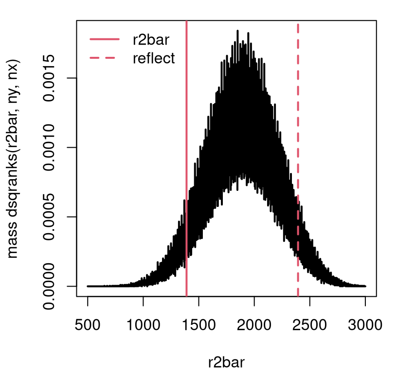
FIGURE 11.1: Exact squared ranks sampling distribution for Metro bikes example.
At first, I thought I had made a mistake with that visual, but it’s correct. Here’s how I know. Consider the special case of \(n_y = n_x = 2\), representing a very small experiment. That means \(n=4\), and so the squared ranks that are available are as follows.
## [1] 1 4 9 16You can’t make any sum of \(n_y = 2\) ranks from those four numbers. There just are six possibilities.
## [1] 5 10 17 13 20 25Anything that’s not one of those numbers would have a mass of zero under the
sampling distribution. That’s a lot of bouncing back and forth, between zero
and nonzero values. By the way, you might think you could short-circuit
some dsqranks calculations by enumerating all nonzero ones via combn. You
can’t, alas, because there are too many for large \(n\) and \(n_y\), e.g., when
\(n = 30\) and \(n_y = 15\) you get get an error from R saying “cannot allocate
vector of size 17.3 Gb”.
Figure 11.1 shows the observed \(\bar{r}^2\) and its reflected
value. The area under the curve in either tail, determining the \(p\)-value,
may be calculated as follows. As implemented, psqranks is merely a sum of
dsqranks.
##     mc  exact
## 0.1188 0.1200
The MC, which is lots simpler in concept and in code, gives a result that’s
quite close to the real thing. Technically speaking, the MC sampling
distribution is just as crazy as the exact one in Figure 11.1.
You wouldn’t be able to tell with a histogram. In fact, the histogram looks
Gaussian! Its bins are obscuring a nuanced relationship. You’d have to count
the number of “hits” for each unique value in R2bars and use a barplot to
see what’s really happening. I encourage you to take a look/give that a try.
Speaking of Gaussians, you might not be surprised that the central limit theorem (CLT) is an option. After all, \(\bar{r}^2\) is a sum, and we already know its mean (11.3). You might also not be surprised that its variance is a nightmare. I’m just going to give you the \(z\) statistic so we can make a quick comparison. Sometimes, this is preferred when there are many ties, and when \(n\) is large. I haven’t found much difference in my own experience.
\[ Z = \frac{\bar{R}^2 - \frac{n_y(n+1)(2n+1)}{6}}{ \sqrt{ \frac{n_yn_x}{n(n-1)} \sum_i r_i^4 - \frac{n_yn_x}{n^2(n-1)} (\sum_i r_i^2)^2 } } \sim \mathcal{N}(0,1) \quad \mbox{ as } \quad n \rightarrow \infty \]
Here that is in code. Note that those sums are over all ranks: \(\sum_i \equiv \sum_{i=1}^n\).
r4sum <- sum(r^4)
r2sum <- sum(r^2)
se <- sqrt(nx*ny/(n*(n - 1))*r4sum - nx*ny/(n^2*(n - 1))*r2sum^2)
z <- (r2bar - R2mean)/se
pval.clt <- 2*pnorm(-abs(z))
pval.clt
## [1] 0.1153This is very close to the others. All three of these options are automated in
the ANSM5 package on CRAN (Spencer 2024), where the test is credited to
Conover (1999). That citation is to the book I learned it from.
However, only the CLT version was provided in that text. Conover only alluded
to an exact option in passing, and didn’t provide any hint of MC. The library
implementation in ANSM5 is a bit different than mine on all fronts. Its MC
calculation is slow and inaccurate. There might be a bug. They make up for it
with a better exact version. Smeeton, Spencer, and Sprent (2025) describe a more purpose-built scheme
for enumerating rank partitions, rather than using a general-purpose SSP
solver. This makes execution much faster, and seemingly no less accurate,
though also an approximation. Finally, their CLT/asymptotic approximation seems
a little off.
library(ANSM5)
pvals <- rbind(
  c(pval.mc, pval.exact, pval.clt),   ## by hand, calculated above
  c(conover(y, x, do.mc=TRUE)$pval.mc, conover(y, x)$pval.exact,
    conover(y, x, do.asymp=TRUE)$pval.asymp)
)
colnames(pvals) <- c("mc", "exact", "clt")
rownames(pvals) <- c("byhand", "lib")
pvals
## mc exact clt
## byhand 0.1188 0.12 0.11528
## lib 0.5830 0.12 0.09483See what I mean about those lib MC and CLT results? Two of these things are
not like the others. Although it’s possible to increase the number of MC
iterations via nsims.mc, that didn’t seem to change the answer much when I
tried it. Another caveat about conover(...) is that it may not perform
exactly the test you requested. Internal logic overrides exact calculation
of \(p\)-values for approximate ones in certain cases, such as when there are
many ties or when \(n\) is large. These rules are sensible, but hard to bypass
in situations where you prefer a particular option in spite of accuracy
concerns or computational cost, like when you’re writing a textbook.
11.2 Kruskal–Wallis
I already said that Kruskal–Wallis (KW) is non-P ANOVA. That means it’s a test for heterogeneity in location across \(m\) samples. Usually \(m \geq 3\) since for \(m=2\) there’s always the Wilcoxon test (§9.2). Specifically, suppose our data consist of \(y_{ij}\), for \(i=1,\dots n_j\) and \(j=1,\dots,m\). We assume that these samples are mutually independent and wish to test if all \(n = \sum_{j=1}^m n_j\) of them come from the same distribution. Or, is it that at least one pair of samples (some \(j \ne k \in \{1,\dots, m\}\)) come from different distribution(s)?
In other words, the hypotheses are like in Eq. (9.2), but for \(m \geq 3\) samples. Alternatively, get rid of the Gaussian in (6.6), and replace \(\mu_j\) and \(\mu_k\), etc., with \(\mathbb{E}\{Y_{ij}\}\) and \(\mathbb{E}\{Y_{ik}\}\), etc. I’m trying to keep it casual and avoid being too pedantic here. KW is a location-based test, and so the test statistic involves aggregated ranks like a Wilcoxon rank sum test (9.3). Yet KW is also like ANOVA in that it uses sums of squares, via a weighted combination of squared average ranks for each group. Don’t worry, I’ll be specific, but I wanted to start by giving you something easier to remember.
Let \(r_{ij}\) denote ranks of the combined sample of all \(n\) observations, with ties yielding averaged ranks as usual. Denote
\[ \bar{r}_j = \sum_{i=1}^{n_j} r_{ij}, \quad \mbox{ for } \quad j=1,\dots,m, \]
as the sum of ranks for each group. Next, combine squares of those rank-aggregates and adjust for their sizes \(n_1, \dots, n_m\).
\[\begin{equation} \bar{r}^2 = \sum_{j=1}^m \bar{r}_j^2/n_j \tag{11.4} \end{equation}\]
I’m using the same letter as for a squared ranks statistic (11.2) because this one is also a sum of squared ranks. Eq. (11.4) is a little different since raw data values \(y_{ij}\) are ranked with KW (targeting location), whereas a squared ranks test involves absolute deviations \(v_i\) and \(u_j\) (targeting scale).
Shocker: \(\bar{r}^2\) in isn’t the only statistic that is used with KW. But it’s the simplest one that allows us to get up-and-running quickly. Others are variations on Eq. (11.4) become more important for asymptotic approximations behind closed-form tests. I’ll get to those later, and pivot here to introducing an example.
Keeping things familiar, a list below collects all Metro fare card
data from §9.2.
ylist <- list(
  VA=c(80, 76, 56, 67, 73, 58, 51, 65, 68, 61),
  DC=c(83, 66, 71, 82, 81, 89, 97, 59, 74),
  MD=c(67, 94, 83, 98, 35, 73, 29, 36, 60, 105, 34, 84, 89, 76, 79, 92,
    49, 97, 46, 32, 104, 60, 61, 59, 98, 101),
  DC2=c(107, 114, 87, 102, 85, 94, 109, 91, 99, 59, 97, 92, 103, 90, 43,
    108, 61, 111, 87, 112, 109, 115, 89, 105, 109, 83, 35, 114))
As with ANOVA, list and data.frame data structures have advantages
when it comes to grouped data. Here, code from §6.3
is borrowed verbatim to extract dimension information, and construct
a data.frame representation.
nj <- sapply(ylist, length)
m <- length(nj)
n <- sum(nj)
ydf <- data.frame(farecards=unlist(ylist), venue=factor(rep(1:m, nj)))
If you recall our separate, pairwise analysis of (VA, DC) and (MD,
DC2) from Chapter 9, you might be able to guess the outcome of the
KW test I’m about to take you through here. Figure 11.2
provides a visual of these data. There are certainly differences between each
of the samples, but it’s not cut-and-dry that they all (don’t) have the same
mean.
boxplot(ylist, border=1:4, ylab="weight")
jit <- rnorm(n, 0, 0.05)
points(as.numeric(ydf$venue) + jit, ydf$farecards, pch=19,
  col=ydf$venue, cex=0.75)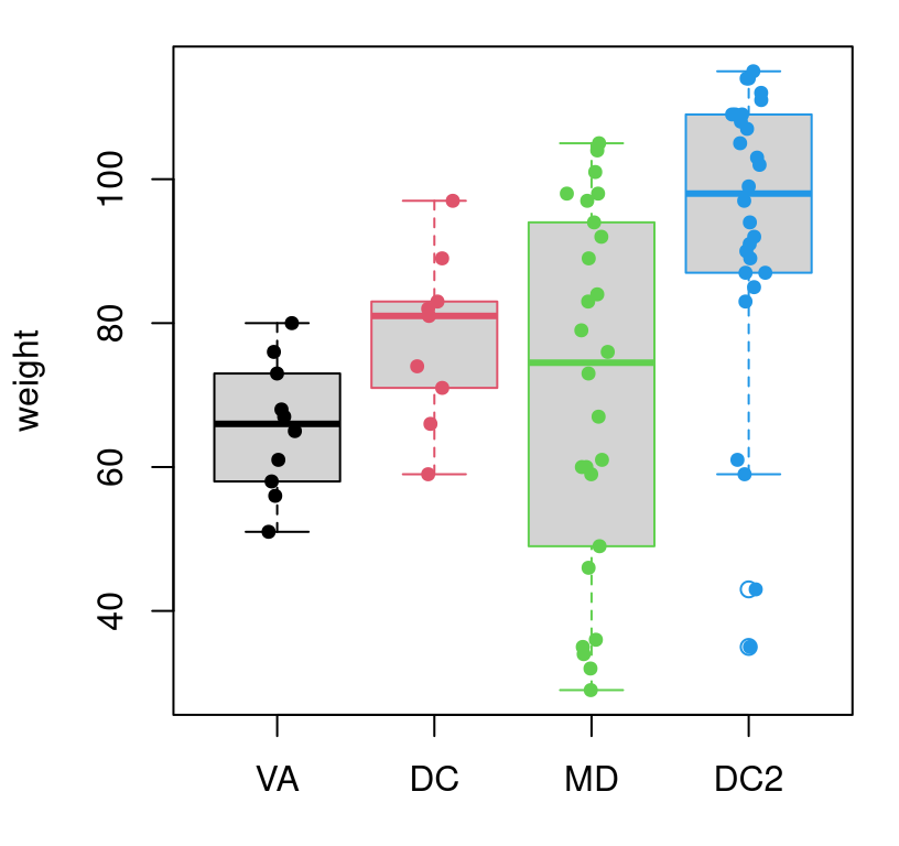
FIGURE 11.2: Visualizing the full Metro fare card data set, with horizontal jitter.
Obtaining ranks for the full data set is easy via unlist.
## [1] 73 50Note that there are a substantial number of ties. Here’s a tidy way to extract ranks for each group or sample, regardless of how many there are, and add them up.
##      1      2      3      4
##  212.5  294.0  777.5 1417.0
I encourage you to take one step at a time through that code and study what each subroutine is doing. It’s not magic. Finally, R code below completes calculation of the test statistic (11.4).
## [1] 109080This is an interesting number. Definitely big! Also it’s nonsense without something to compare it to.
KW test via MC
As always, just be careful to follow the statistic (11.4) under the null hypothesis, which in this case – as it has been with all methods based on ranks – is based on uniform permutation. Generate random ranks by sampling indices \(\{1,\dots, n\}\) without replacement, break them into \(m\) groups of size \(n_1, \dots, n_m\), sum within each group, and then aggregate their squares weighted by inverse sample size.
for(i in 1:N) {
  Rs <- sample(1:n, n, replace=FALSE)       ## random permutation
  Rgs <- tapply(Rs, g, sum)                 ## break into groups and sum
  R2bars[i] <- sum(Rgs^2/nj)                ## calculate statistic
}
Without acknowledging ties, this virtualization is not completely faithful to
the conditions under which our Metro fare card data was observed. As with
squared ranks, you may easily mimic observed ties with rand.ties, but I’m
skipping that here to keep things moving. Since the statistic is a square,
the sampling distribution will have positive support and be heavily
right-tailed. See Figure 11.3. In such situations, the test is
implicitly one-sided, just like ANOVA. Any small value of \(\bar{r}^2\)
supports the null.
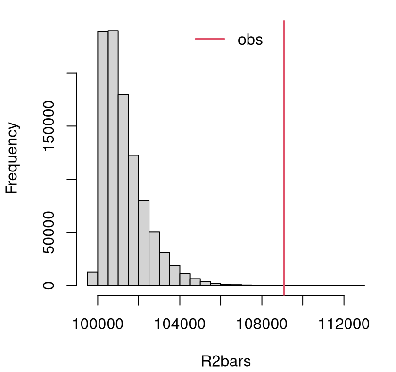
FIGURE 11.3: Empirical sampling distribution of \(\bar{R}^2\) for KW on Metro fare card data.
The figure indicates a clear reject, but the additional precision offered by \(p\)-value never hurts.
## [1] 5.5e-05Since two of the pairs of samples led to rejections of the null in Chapter 9, the outcome here is not surprising: at least two of the samples differ in their mean. As always with an ANOVA-type analysis, one can pair off to find the culprit after a rejection. In this case – because of the order I thought it best to organize material into chapters – we’ve done that already. Perhaps that makes this example a little boring, but you’ll have the opportunity to try others in your homework.
KW test via math
One may, technically speaking, use an SSP-based counting routine to derive mass and distribution for \(\bar{r}^2\) exactly. However, considering the magnitudes involved (\(\bar{r}^2 = 1.0908\times 10^{5}\)), that would represent a computationally daunting undertaking. Instead, an asymptotic approach is favored.
It can be shown that
\[\begin{equation} X^2 = \frac{\bar{R}^2 - \frac{n(n+1)^2}{4}}{ \frac{1}{n-1}\left[\sum_{j=1}^m\sum_{i=1}^{n_j} r_{ij}^2 - \frac{n(n+1)^2}{4}\right]} \sim \chi^2_{m-1} \quad \mbox{ as } n \rightarrow \infty. \tag{11.5} \end{equation}\]
In the case of no ties, the denominator above reduces to \(n(n+1)/12\). On the face of it, that might seem helpful for by-hand calculations. On the other hand, if you can calculate \(\bar{r}^2\), then it stands to reason that you can sum up and square all \(n\) ranks without issue. So perhaps that cute result is mere trivia. I’m not going to prove any part of Eq. (11.5) to you, but I’ll show it to you in action.
## [1] 20.32One nice thing about this number, as opposed to \(\bar{r}^2\), is that it has a higher degree of interpretability. \(\chi^2_{m-1}\) distributions have a mean and variance of \(m - 1\) and \(2(m-1)\), respectively. With \(m=4\) that makes \(x^2 = 20.32\) point to an easy reject at 5% since that’s 3 standard deviations away from the mean. A \(p\)-value works too.
##        mc      asym
## 0.0000550 0.0001456
ANSM5 on CRAN offers the only packaged option for comparison that I’m aware
of. Although its kruskal.wallis routine has a do.exact=TRUE option, that
choice only works for problems where \(n\) is small. Here small means \(n \leq\,\)
max.exact.cases=15 by default. Increasing to max.exact.cases=n results in
a memory allocation error. Consequently, the only (other) library options are
MC and asymptotic calculations, just like those above.
yflat <- unlist(ylist)  ## so code below will fit horizontally
c(lib.mc=kruskal.wallis(yflat, g, do.mc=TRUE, nsims.mc=100000)$pval.mc,
  lib.asym=kruskal.wallis(yflat, g, do.asym=TRUE)$pval.asymp)
## lib.mc lib.asym
## 0.0000400 0.0001456That’s close in the first case and exact in the second. Notice that I upped
the number of MC simulations so that the result would more closely resemble
those from my bespoke loop above. I wasn’t able to do nsims.mc=N; that was
too big of an ask to return a result in a reasonable amount of time.
Note that the SuppDists on CRAN (Wheeler 2025) provides a pKruskalWallis
function, promising a cdf evaluation. However, I’ve been unable to figure out
from its documentation how it can be used in a KW test using a setup that was
familiar to me. Perhaps I haven’t been patient enough with it, since other
functions from that library have come in handy; see Chapter 12.
An astute observer will notice that the asymptotic sampling distribution for squared ranks – a test of scale – uses a Gaussian approximation while KW – a test of location – uses \(\chi^2\). I find this puzzling, since Gaussians are location models and \(\chi^2\) are scale. The KW result is consistent with ANOVA-like procedures, so perhaps it’s squared ranks that’s the odd duck.
11.3 Homework exercises
These exercises help gain experience with squared ranks and Kruskal–Wallis tests. There are no math questions this time; all are coding and/or data analysis. Don’t forget to try each test multiple ways, e.g., via MC and math/asymptotics. If you’re looking for more practice, any questions on P-based tests of variance and ANOVA from §6.5 are appropriate as well. Needless to say: my intention here is that you use a non-P test.
Do these problems with your own code, or code from this book. Unless stated explicitly otherwise, avoid use of libraries in your solutions.
#1: Ties in ranks
Repeat the Metro fare card example with KW, except augment your MC to respect
ties in the ranks via rank.ties in
rank_ties.R.
#2: monty.sqrank and monty.kw
Write library functions for all methods in this chapter. That means
squared ranks and KW via MC, exact, and asymptotic calculations. Since they
are different tests for distinct situations, I suggest two separate functions.
Optionally incorporate your rank.ties solution from #1, which may
additionally include support for KW. Feel free to use any of the code in
ranks.R.
Hint: many of the following questions are easier after this one is squared away.
#3: Outside temperature
Measurements below provide the highest recorded temperature in degrees Fahrenheit for Blacksburg, VA and Arlington, VA on several randomly sampled days in one summer.
bburg <- c(75, 82, 80, 85, 77, 90, 83, 85, 88, 89, 81)
arlington <- c(88, 81, 96, 76, 98, 79, 81, 82, 88, 93, 91, 85, 84, 90)
Is variability in temperatures at these VA locations different?
#4: Inside temperature
As part of a survey on personal comfort, participants were asked to report their gender (recorded as male and female), among other information, and their ideal winter-time room temperature in degrees Fahrenheit. A subset of those values are provided below.
male <- c(65, 73, 69, 71, 68, 69, 70, 67, 71, 65, 72, 67, 69, 65,
  66, 68, 67)
female <- c(70, 69, 70, 68, 68, 69, 71, 70, 68, 69, 69, 70, 71, 69)
Is there a difference in variance for indoor temperature comfort level for these two groups?
#5: Return on investment
Refer back to roi$company and roi$industry from §2.5.
Recall that these data are available as
roi.RData on the book webpage.
Is there any difference in ROI variance between companies that use the IT product in question and the industry at large?
#6: TV watching
Student researchers at a liberal arts college asked other randomly selected students questions about their TV-watching habits. They divided their subjects into four groups: male athletes (MA), male non-athletes (MNA), female athletes (FA), and female non-athletes (FNA). These data, recording hours watched per day, may be found on DASL, or as tv.csv on the book webpage.
What do you think? Are TV-watching habits differentiated by gender and
athletics? Hint, repeated from §6.5: one convenient
way to turn two vectors, one with real-valued measurements and another
factor grouping variable, is with split in R.
#7: Hand-washing
A student studied four methods for eliminating bacteria via hand-washing: water only, with regular soap, with antibacterial soap (ABS), and spraying hands with an alcohol-based antibacterial spray (AS; containing 65% ethanol as an active ingredient). These data, counting bacteria on participants’ hands after an incubation period, may be found on DASL, or as bacteria.csv on the book web page.
What do you think? Is the level of effectiveness about the same for all four
methods? (See split hint above in #6.)
#8: Light bulbs
Light bulb manufacturers boast longer lifetimes for LEDs compared to classical incandescent and compact-fluorescent (CFL) bulbs. This is generally true in controlled settings like leaving them on continuously. Things are more complicated with everyday home use where they’re turned on-and-off several times per day. Data values below record lifetimes in months for three kinds of bulbs from a single manufacturer.
bulbs <- list(
  incan=c(73, 69, 66, 72, 66, 70, 85, 73, 79, 92),
  cfl=c(83, 90, 81, 83, 100, 68, 77, 71, 78, 95),
  led=c(84, 102, 79, 98, 75, 102, 115, 74, 58))
Is there any difference in their lifetimes?
References
ANSM5: Functions and Data for the Book “Applied Nonparametric Statistical Methods,” 5th Edition. https://doi.org/10.32614/CRAN.package.ANSM5.
SuppDists: Supplementary Distributions. https://doi.org/10.32614/CRAN.package.SuppDists.