Chapter 2 Location: mean modeling

According to search results I got when I Googled “United States height average and standard deviation”, adult American women are about 64.5 tall inches with a standard deviation of 2.5 inches. Suppose you surveyed women in your stats class and obtained \(n\) height measurements, in inches. Now you “want to know”, are women in your class similar to adult women in the USA at large? In particular, do they have the same average height?

I encourage you to do this with data collected from your class, or other women you know. I’m not going to guess at what you got. Here’s some data from when I ran this experiment with one of my classes.

y <- c(65, 65, 69, 67, 66, 66, 67, 64, 68, 68, 68, 69, 70, 65, 70, 
  67, 65, 62, 69, 68, 65, 68, 64, 64)
n <- length(y)

In the remainder of the chapter I shall answer this question using tools from Chapter 1, along with a new modeling construct based on a particular example of location models, which are a special case of the location–scale family of probability distributions. I aim to show you that you basically know how to do this already. So we’ll be able to move through things quickly, although like with coin flips some detail will be tabled for later.

2.1 Modeling

Technically we have data from two populations: adult US women and women in my class. For now, let’s assume the survey of women in the USA was very large, and so we may take the mean and standard deviation estimates from that population as accurate proxies for the gold-standard truth. In other words, the mean height of women in the USA is \(\mu = 64.5\), and the standard deviation is \(\sigma = 2.5\).

mu <- 64.5
sigma2 <- 2.5^2  ## for sigma^2; more on that in a moment

Quick digression on means versus averages, which are estimates of means. They’re not the same thing. One (mean) refers to a population quantity, like \(\mu = \mathbb{E}\{Y\}\), where \(Y\) is a random variable representing American women’s heights. The other (average) is an estimate obtained from a (possibly small) \(n\)-sized sample from that population. They’re not the same unless you sample everyone in the population, i.e., if \(n = 168\) million, according to Google. I just wanted to make sure that’s clear before we move on.

To possibly muddy the waters, I’m taking a number I got from Google and treating it as a mean. Google is almost certainly providing an average from a small, or modestly sized, sample. They didn’t ask everyone, and for the purposes of the example I am treating an estimate as a population quantity: a mean \(\mu\), and a variance \(\sigma^2\). I’m doing this to compare it to students in my class, who are clearly a much narrower (and possibly not representative) sample of the larger sample, and of the population. Partly, I’m doing this because we’re not yet equipped to deal with two samples yet. That’s Chapter 5. Hold your horses.

Alright, back to modeling. The first step of any statistical inference exercise is to specify a probabilistic model for the data, our 24 measurements in y. We chose a Bernoulli model for coin flips in Chapter 1, and now we need something appropriate for heights in inches. In other words, we need a probability distribution for how heights, such as those observed for American women, could have been generated. We don’t need to believe this is how they were generated, because of course that’s preposterous. No model will be perfect, and ultimately this is a choice of convenience. We want something that is not egregiously wrong. Moreover, it helps to choose a family of distributions that can be “matched up” with the information we have, summarized by \(\mu\) and \(\sigma^2\).

Suppose we assume that adult heights are Gaussian, i.e., that they follow a so-called normal distribution. This is easy to quibble with, but not ridiculous. For one thing, you’d never get any duplicates if that were the case, and there are some duplicated heights in y. That’s a more involved discussion for later; we’re still in the warm-up phase of the book. Again, this isn’t a text on probability, which I presume you already have some experience with. If not, that Wikipedia link should help. I’ll provide some of the necessary detail here, and more in later chapters.

If we notate each measurement as \(y_i\), with random analog \(Y_i\), then we may characterize our model for \(n\) independent and identically distributed measurements as follows,

\[\begin{equation} \mbox{Model:} \quad\quad Y_1, \dots, Y_n \stackrel{\mathrm{iid}}{\sim} \mathcal{N}(\mu, \sigma^2), \tag{2.1} \end{equation}\]

where parameters \(\mu\) and \(\sigma^2\) dictate the shape of the bell curve of the Gaussian density function. Parameter \(\mu\) determines the center of the density, or location, and can take on any (finite) real value. It specifies the mean: \(\mathbb{E}\{Y_i\} = \mu\). Parameter \(\sigma^2\) determines the spread, with, or scale of the bell. It also determines the variance: \(\sigma^2 = \mathbb{V}\mathrm{ar}\{Y_i\} = \mathbb{E}\{(Y_i - \mu)^2\} = \mathbb{E}\{Y_i^2\} - \mathbb{E}\{Y_i\}^2\). Without the square, \(\sigma\) is known as standard deviation. You may recall that about 95% of \(Y_i\) values lie within \(\mu \pm 2\sigma\) under a Gaussian distribution.

I want to assume a Gaussian could characterize the height of a random woman in the USA, i.e., \(Y \sim \mathcal{N}(64.5, 2.5^2)\) using mean and standard deviation information gleaned from a Google search. Figure 2.1 shows what that bell curve looks like. The mathematical convention is to notate variances \(\sigma^2 \equiv\) sigma2 (in code), especially for Gaussian distributions. In R, however, standard deviation is used for dialing in the density of a normal/Gaussian distribution. So you’ll see in the code that I’m always careful to use the number 2 in my variable name for \(\sigma^2\) (i.e., sigma2), but then I take the square root of that quantity to pass it to dnorm, the density function. You’ll probably find that to be pedantic, but it’s a great way to avoid bugs. Take my word for it.

ygrid <- seq(50, 80, length=1000)
plot(ygrid, dnorm(ygrid, mu, sqrt(sigma2)), type="l", 
  xlab="y", ylab="density N(64.5, 2.5^2)", lwd=2)
points(y, rep(abs(rnorm(n, 0, 0.005))))
abline(v=mu + c(-2, 2)*sqrt(sigma2), col=2, lty=2, lwd=2)
legend("topright", "observed", pch=21, bty="n")
legend("topleft", "95%", col=2, lty=2, lwd=2, bty="n")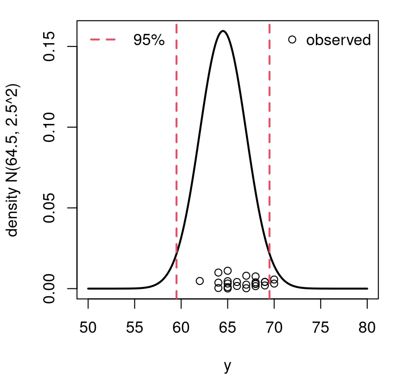

FIGURE 2.1: Visualizing data on women’s heights from class versus the US population of women’s heights at large. Vertical jitter is added to more easily see duplicated heights.

Overlayed on the density plot in the figure are the 24 observed measurements from women in my class. Basically the “want to know” question boils down to: could it be that those \(n= 24\) heights, from my class, were drawn from the same distribution as women in the USA as characterized by the density drawn on the plot? Visually, it doesn’t seem implausible. Sure, the observed values concentrate a little to the right of \(\mu = 64.5\). And, 8% of them are outside of the 95% interval, which is a little high (only 5% should). But it’s not too crazy, right?

How can we make a call in a more principled, and precise manner? How likely is it to see data that we got by chance, in my class, as opposed to anywhere else? Are women taking stats at VT special? (They will be once this class is over! Though not because of their height. They’ll have mad stats skills!)

Quick digression before answering that question. People use “Gaussian” and “normal” interchangeably, and so will I. They mean the same thing. There are other members of the location–scale family; and there are many good choices of outside that family where you can still match moments to \(\mu\) and \(\sigma^2\) to set parameters. You’ll get to tinker with that in the homework exercises of §2.6. My particular Gaussian choice here simplifies many matters, which again I’ll return to later.

Alright, back to testing, but I need one last thing. In what follows, I’m going to make a common “baby steps” simplifying assumption that the standard deviation (or variance) is known, and fixed to \(\sigma^2 = 2.5^2\) for all heights of women regardless of population. This is not correct, and I will fix it in §3.1. For now, it allows me to focus our investigation on mean \(\mu\), on location.

2.2 Testing apparatus

We have our data and our model. We need to clarify hypotheses and choose a testing statistic. Then we can follow Alg. 1.1 via Monte Carlo (MC), just like in Chapter 1. I wish to know if the mean from my class is the same as the mean from the population at large. That can be written as a set of competing hypotheses much in the same way as Eq. (1.4).

\[\begin{align} \mathcal{H}_0 &: \mu = \textstyle 64.5 && \mbox{null hypothesis (``what if'')} \tag{2.2} \\ \mathcal{H}_1 &: \mu \ne 64.5 && \mbox{alternative hypothesis} \notag \end{align}\]

That’s the easy part. The harder part, and where it can help to be creative, is to choose a test statistic \(s_n\). Recall that it is the sampling distribution of \(S_n\), contrasted against observed \(s_n\), which plays an integral role in a contradiction argument behind the process of Alg. 1.1. I bet you already know what statistic you want to use: the sample average \(s_n = \bar{y}_n = \frac{1}{n} \sum_{i=1}^n y_i\). The sample average is an estimator of the mean, a topic we’ll return to in more detail in §3.2, and the mean \(\mu\) is the focus of our hypotheses (2.2). Almost certainly, the sample average will differ from the value of \(\mu\) specified by the null hypothesis; therefore, it supports the alternative \(\mathcal{H}_1\).

s <- mean(y)
s

## [1] 66.62

If intuition is failing you, or if it brought you down some other path (there are plenty of reasonable choices!), let me again whet your appetite for §3.1. There, I’ll provide an automatic method for choosing a test statistic \(s_n\) for tests that are based on parameters describing distributions underlying the data-generating model (2.2). For now, allow me to appeal to reasoning that an estimate (sample average) is a good proxy for a population quantity (mean). If fact, it’s so good that people often believe they are one and the same thing when they’re not, hence my disclaimer earlier, at the start of the chapter.

Quick digression to foreshadow a little and indulge in a couple of quick technical explanations for why the sample average is a good test statistic for the mean. Under a Gaussian distribution, each \(\mathbb{E}\{Y_i\} = \mu\), for all \(i=1, \dots, n\). By linearity of expectations, the expected value of a (weighted) sum of random variables is equal to the sum of their expected values. We can use that with \(S_n = \bar{Y}_n\).

\[\begin{equation} \mathbb{E}\{S_n\} = \mathbb{E}\left\{\frac{1}{n} \sum_{i=1}^n Y_i \right\} = \frac{1}{n} \sum_{i=1}^n \mathbb{E}\{ Y_i \} = \frac{1}{n} \times n\mu = \mu. \tag{2.3} \end{equation}\]

In other words, the expected value of the statistic is equal to the parameter of interest. We say that the sample average is an unbiased estimator for the mean. Eliminating bias is a good thing, especially in a data-poor situations. So the sample average has one feather in its cap.

Let’s look at the variance of our statistic. Under a Gaussian distribution, each \(\mathbb{V}\mathrm{ar}\{Y_i\} = \sigma^2\) for all \(i=1, \dots, n\). By linearity of variance, the variance of a (weighted) sum of independent random variances is the sum of the (squared weights) variances. For us:

\[\begin{equation} \mathbb{V}\mathrm{ar}\{S_n\} = \mathbb{V}\mathrm{ar}\left\{\frac{1}{n} \sum_{i=1}^n Y_i \right\} = \left(\frac{1}{n}\right)^2 \sum_{i=1}^n \mathbb{V}\mathrm{ar}\{ Y_i \} = \frac{1}{n^2} \times n\sigma^2 = \frac{\sigma^2}{n}. \tag{2.4} \end{equation}\]

So as \(n\) increases, the variance of \(S_n\), which is the same as its squared expectation around its mean (and which we just learned is \(\mathbb{E}\{S_n\} = \mu\)), decreases. If you’re following along with those Wikipedia links, note that the \(\mathbb{C}\mathrm{ov}\) term you see on that page is not present in Eq. (2.4) because I assumed independence. Independent random variables do not co-vary; they have a covariance of zero.

Whenever information goes up (e.g., from more data \(n\)) and uncertainty goes down (2.4), that means you’re learning something! So \(S_n\) is good for \(\mu\) because it is unbiased, and because it extracts information, decreasing uncertainty with \(n\). Observe that as \(n \rightarrow \infty\) we have that \(\mathbb{V}\mathrm{ar}\{S_n\} \rightarrow 0\). Eventually, with enough data \(n\), \(S_n\) reveals \(\mu\) precisely, and without uncertainty. This is not true of all choices of \(S_n\).

For example, what if we chose \(S_n = Y_1\)? That is, just estimate that the mean is equal to the value of the first observation, ignoring the other \(n-1\). This might seem silly, but it has some good properties. It is unbiased since \(\mathbb{E}\{ Y_1\} = \mu\). But it does not do a good job of extracting information: \(\mathbb{V}\mathrm{ar}\{ Y_1 \} = \sigma^2 \ll \frac{\sigma}{n}\) for all \(n > 1\). No matter how much data you gather, \(n\), you’ll never learn \(\mu\) with improved precision.

There is a sense in which \(S_n = \bar{Y}_n\) is optimal for \(\mu\) under a Gaussian distribution because it minimizes mean-squared error (MSE). MSE is a hybrid statistic that combines bias and variance in a particular way. But that’s a technical topic that is best left for a more advanced text.

Alright, back to the task at hand. We’ve been able to use some math to understand the central moments of \(S_n\). But we need the whole sampling distribution to adjudicate between hypotheses in Eq. (2.2).

2.3 Sampling distribution

In fact, you can use math to work out the sampling distribution in closed form. It’s not terrible, but you guessed it: I’ll delay that until §3.2. Because it’s much simpler, and more easily adjusted to other settings, we’ll instead simulate here from the sampling distribution by MC. The model is Gaussian (2.1), so all you have to do is repeatedly draw \(n = 24\) \(Y_i\)-values from a Gaussian pseudo-random number generator and save averages. Here we go.

N <- 10000                          ## number of MC "trials"
Ss <- rep(NA, N)                    ## storage for sampled test stats
for(i in 1:N) {                     ## each MC trial
  Ys <- rnorm(n, mu, sqrt(sigma2))  ## change 1: generate n Gaussian samps
  Ss[i] <- mean(Ys)                 ## change 2: calculate test stat
}

Note that there are only two changes to the MC for coin flips in §1.3. It bears repeating: be careful to take the square root of \(\sigma^2\) when using R’s normal generators (or density functions, or anything else). This is a common source of bugs in code even for seasoned R professionals. When coding in-real-time, or under the pressure of being at a projector in front of class, I make this mistake all the time. You can score some brownie points with your professor by helping fix a problem like this by calling it out before it really becomes one.

What to do with those samples? The same exact thing we did for coin flips. Once we have samples from the sampling distribution for \(S_n\), we can (optionally) visualize them to contrast with observed \(s_n\), or jump straight to a two-tailed \(p\)-value calculation. Figure 2.2 shows a view of the empirical distribution, overlaying \(s_n\) and its reflection over the mean as vertical lines. Again, empirical distributions are covered in more detail in §A.1. Here, I just mean that the histogram is summarizing a spread of sampled values, showing how they distribute on the \(x\)-axis.

hist(Ss, main="", xlim=range(s, 2*mu - s, Ss)) 
abline(v=c(s, 2*mu - s), lty=1:2, col=2, lwd=2)
legend(65, 1650, c("s", "reflect"), col=2, lty=1:2, lwd=2, bty="n")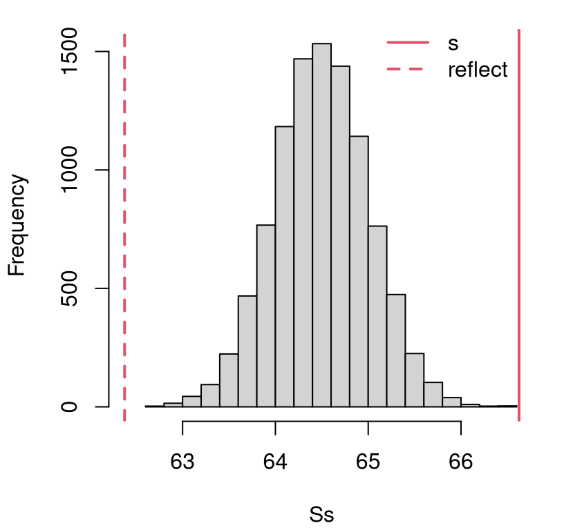

FIGURE 2.2: Histogram of samples \(S_n\) from their sampling distribution under \(\mathcal{H}_0\), and the actual \(s_n\) (and it’s “two-tailed” reflection) for comparison, for the heights experiment.

A simple, means-based reflection is fine since Gaussians are symmetric. This involves finding the value which is the same distance from the middle of the distribution as \(s_n\) is, but put it on the other side. Notice I used mu for the reflection instead of mean(Ss). Both work and are correct, but mu is more accurate for finite MC effort \(N\) since I already know that \(\mathbb{E}\{S_n\} = \mu\). That was the basis of our argument that \(S_n\) is unbiased (2.3). Any time you can use something that you know is exact, mathematically, as opposed to being calculated via MC you’ll get a more accurate calculation. I encourage you to try swapping out for 2*mean(Ss) - s instead.

Clearly both \(s_n\) and its reflection represent unlikely observations under the null hypothesis. It doesn’t look like any of our \(N = 10{,}000\) simulations of \(S_n\) is more extreme than what we observed in the data. This means that a calculation in R for the \(p\)-value with these samples will show zero.

pval <- mean(Ss < 2*mu - s) + mean(Ss > s)
pval

## [1] 0

That isn’t quite right, without acknowledging that the calculation is sensitive to the amount of MC sampling effort \(N\). A better answer is that the \(p\)-value, often notated as \(\psi\), in this case follows \(\psi \leq 1/N \lessapprox10^{-4}\). If your threshold is \(\alpha = 0.05\) then even without that improved precision you’ve got a pretty clear reject of \(\mathcal{H}_0\), and no further action is necessary.

Based on this, I conclude that women in my class are not like the population at large, at least not based on their height. I can probably explain that on socioeconomic grounds. Women who attend college are more affluent than those who do not, which means better nutrition among other things, so they’re likely to be taller. Yet that sort of thing is an indulgence without further information. It’ll be fun to ponder such things in this book, but I’m not serious about it. (I am serious about the stats though!)

If you want more precision out of an MC \(p\)-value calculation, increase \(N\) and keep going. I had to increase \(N\) one-hundred-fold to get more than one hundred extreme values. Your mileage may vary as you’ll get different random draws than me.

N2 <- N*100
Ss <- c(Ss, rep(NA, N2-N))                  
for(i in (N+1):N2) {                       
  Ys <- rnorm(n, mu, sqrt(sigma2))        
  Ss[i] <- mean(Ys)                   
}
p100 <- mean(Ss < 2*mu - s) + mean(Ss > s)
p100

## [1] 2.6e-05

Finally, since Gaussians are symmetric, so will be the sampling distribution. More detail is available in Chapter 3. This means that we’ll get the same \(p\)-value, up to error inherent in a small MC sample, by doubling a one-tailed \(p\)-value.

2*mean(Ss > s)

## [1] 3e-05

However, if you don’t know for sure that your sampling distribution is symmetric, then you can always do the following instead. Calculate the empirical quantile of \(s_n\) in the distribution for \(S_n\), and then match it with a value in the opposite tail.

pl <- mean(Ss >s)
sr <- as.numeric(quantile(Ss, pl))
c(dist=2*mu - s, quantile=sr)

##     dist quantile 
##    62.38    62.42

They’re not the same, but pretty close. The quantity s lies in some percentile of Ss, which may be calculated as mean(S > s), and in this case lies in the right tail (implicitly pr). One minus that is pl = mean(Ss >= s) in the left tail. The command quantile(Ss, pl) extracts the value of Ss that lies the pl percentile: the equivalent extreme value observed in the opposite tail of the sampling distribution. So the reflection sr is like the left-tail image of the statistic we observed in the right tail, in this instance. The idea is that the statistic and its reflection have the same amount of (more extreme) tail probability.

Then calculate the \(p\)-value as follows.

mean(Ss < sr) + mean(Ss > s)

## [1] 3e-05

So we get the same thing as doubling the one-tailed \(p\)-value. It’s that way by construction. We made it so the quantiles match exactly.

2.4 Wrapping up

See, that wasn’t so bad. It’s basically the same thing as in Chapter 1 except with a different distribution – one appropriate for real-valued measurements. In Chapter 1, I built a library function and then compared to calculations built into R. Some of the details involved in finding a reflected statistic for a two-tailed \(p\)-value were buried in a subroutine because of the discrete, asymmetric nature of the sampling distribution.

This time it’s easier because of symmetry, so I’m going to let you make the library function as a homework exercise. I suggest calling it monty.z. What we’re doing here is known as a \(z\)-test. The reason for this is that (standardized) Gaussian deviates, which is another name for random variable, are often notated with the letter \(Z\) or \(z\). You may have heard of a \(t\)-test, which is the generalization of a \(z\)-test. A \(z\)-test uses a known variance \(\sigma^2\), whereas a \(t\)-test uses estimated \(\sigma^2\) and consequently differs in a few other details. Wait for Chapter 3.

These \(z\)-tests are a great place to start – often right after binomial tests but sometimes the other way around – because they’re relatively simple. They’re not particularly common in practice, at least for data under a Gaussian model, because usually you do want to estimate \(\sigma^2\). There’s no \(z\)-test built into R, but you can get one from a library on CRAN. There are many, and I have chosen one from the BSDA (Basic Statistics and Data Analysis) package (Arnholt and Evans 2023) somewhat arbitrarily.

## install.packages("BSDA")  ## only do this once per machine
library(BSDA) 
z.test(y, mu=mu, sigma.x=sqrt(sigma2))$p.value

## [1] 3.125e-05

Observe that this \(p\)-value is similar to the second one calculated above, based on \(N= 10^{6}\) MC samples. Note that you only need to install an R package once per machine, but it must be loaded with the library command each time you start a new session. Since I have already installed the package, the install.packages command is commented out above. You’ll need to do that (un-comment it, once on your machine) if you haven’t already.

2.5 Return on investment

I used to work in the Booth School of Business teaching MBAs at The University of Chicago. When I started working there, some colleagues passed me a cool data set that was tied to a statistical analysis provided by a major consulting company. The clients of that company based an aggressive, negative advertising (smear) campaign against their competition, on that analysis. I’m being a little coy here not to mention the names of these companies, or the statistical consultancy, because I don’t want anyone annoyed at me. But I am going to share the data involved in that analysis with you, because you can do (a better job of) that analysis. It’s not that hard. Find the file as roi.RData on the book webpage.

load("roi.RData")    ## defines variable roi, which is a list
roi

## $company
##  [1]  21.1  15.8   1.2  61.2  15.2  26.4  66.9   5.4  12.2   4.9  20.8
## [12]  23.3  13.2  14.5  27.3  17.0 -41.1  35.9 116.4   8.1   7.9   6.7
## [23]  32.7  11.6  17.1 -47.5  23.8   1.1  26.7   6.9  13.4  14.9  14.9
## [34]  14.6 -15.4   4.6  43.9  15.8   6.4  13.1  14.6   8.4   8.9   8.8
## [45]  23.1 -91.8  45.8   7.3  18.9  22.8  -7.7   6.8  -9.2 -62.6  18.7
## [56]  27.3   8.3  16.7  18.4  28.8  25.6  16.9   0.3  -0.7 -38.5   8.3
## [67]   8.3   8.3   8.3   6.2   6.2  -0.5  18.6   0.9  47.4  27.3   4.7
## [78]   2.8  41.4  26.0  14.6
## 
## $industry
##  [1]  8.7 19.5 19.5 22.0 19.6 22.2 10.6  3.7 19.5 22.2 14.0 11.9 14.9
## [14]  8.8 18.2 10.2 16.3 15.3 14.9 10.9 10.9  9.8  9.5  6.4 15.3 13.3
## [27] 20.2 26.0 26.1 14.0  8.6

These are real data about real companies. I verified that with some of my own digging, at first not trusting the narrative of my colleagues. It used to be that you could download a PDF document containing these data from the website of the statistical consultancy. They were proud of these data and their analysis. Now you can’t find it anymore, or at least I couldn’t. I won’t speculate why, but I can insinuate by helping you conduct some analysis of your own. These data focus on a financial variable called return on investment (ROI). Higher ROI is better. In a down-year for sales, say, it might be low or negative. If ROI doesn’t (eventually) trend positive on aggregate, year-on-year, then the company isn’t going to stay in business long.

When you run that load command, your environment is populated with an object called roi that is comprised of an R list object with two vectors. One contains ROI numbers for particular companies that use a particular IT product that I won’t name. These are found in roi$company. There is one number for each company. Think Apple, Google, Bayer and AstraZeneca, which may or may not have been part of the study. The other vector, roi$industry, contains similar ROI numbers for the sectors that these companies operate in. Think of these numbers as aggregate ROIs for all of the companies in that industry. There would be one for high tech companies (Apple, Google) and one for pharma (Bayer, AstraZeneca), for example and among others.

Figure 2.3 provides a visual of these two, related data sets. The first thing folks notice is that the spread of values for $industry is much narrower than $company. This makes sense because the former is based on an aggregate – on all companies in a particular industry – and the latter are single companies representing part of that whole. Since not all companies use the particular IT product in question, there are some companies represented in the $industry aggregate that are not represented in the $company vector.

hist(roi$company, main="", xlab="ROI") 
hist(roi$industry, col=2, add=TRUE)
legend("topright", c("company", "industry"), fill=c("gray", "red"), 
  bty="n")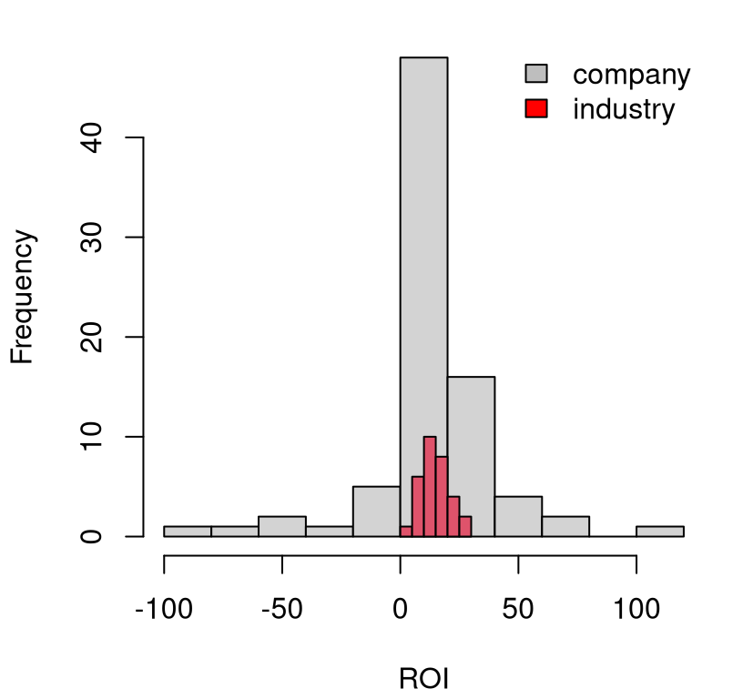

FIGURE 2.3: Histogram of ROI for individual companies and the industries they are part of, at large.

The other thing folks notice is that the entire red histogram is positive. This also makes sense. These industries make money. If they didn’t, they would collapse. Individual companies, with their much wider spread of ROIs, have more extreme values, particularly negative ones.

The focus of the consultant’s statistical analysis, and their client’s subsequent advertising campaign involved sample averages.

ybar <- c(com=mean(roi$company), ind=mean(roi$industry))
ybar

##   com   ind 
## 12.64 14.94

From these you can see that it’s less profitable to be a company who uses a particular IT software than it is to be a company in the population at large. By taking the ratio of the first number over the second, the consultancy concluded that companies using that IT software were 15% less profitable. Their client pounced on this and proclaimed, on billboard advertisements at bus stops and subway stations, that “Companies who use XXX are 15% less profitable than their peers”. Quite a smear.

Is it true? Taking some sample averages and dividing them is a statistic, but it is not doing Statistics, capital “S”. What are the chances that you could get a ratio like that by pure chance? Could it be that the $company population actually has the same mean as the $industry at large? Can we reject that hippopotamus?

I’ll let you decide in a series of homework problems, some in this chapter and some in later chapters. We’ll start simple and then build up sophistication. I’ll give you a little spoiler alert: the evidence isn’t very compelling. It’s a wonder nobody was sued. Maybe they settled out of court.

2.6 Homework exercises

These exercises help gain experience with \(z\)-tests, and extensions, for location. We shall return to some of them later with an expanded toolkit.

Ensure that you are using methods outlined in this chapter. Many students will have experience working with \(z\)-tests in other contexts, from previous classes, other books, or materials found online. Those will be discussed and evaluated in later chapters and homeworks. Deploying non-Chapter 2 methods here will likely not earn full credit.

Do these problems with your own code, or code from this book. In some cases you can check your work with z.test from BSDA. However, check with your instructor first to see what’s allowed. Unless stated explicitly otherwise, avoid use of libraries in your solutions.

#1: Library function

Write a library function like monty.bern from §1.4 but for testing \(\mu\) with observations modeled as Gaussian with a particular, fixed \(\sigma^2\) parameter. Call it monty.z. Include optional visuals when vis=TRUE and return a similar list of relevant quantities.

#2: Fewer heights

What would you conclude for the women’s heights experiment if, on the particular day the data was collected, fewer women came to class. That is, suppose you got …

• y14 <- y[1:14] ## (first fourteen women)
• y7 <- y[1:7] ## (first seven women)

#3: Logistic distribution

Revisit the (full) heights data but instead of a Gaussian distribution, use a logistic distribution, which is another member of the location–scale family. The logistic has two parameters, mean \(\mu\) and scale \(\sigma\) (notated as \(s\) on that Wikipedia page). The mean has the same interpretation as the Gaussian, where \(\mathbb{E}\{Y_i\} = \mu\) for all \(i=1,\dots,n\). But \(\sigma\) is not the standard deviation. Wikipedia explains that \(\mathbb{V}\mathrm{ar}\{Y_i\} = \sigma^2 \pi / 3\). It probably won’t escape you that \(\pi / 3 \approx 1\), but not exactly. So you’ll need to do a little work to use standard deviation information from the US population of women with the logistic parameter \(\sigma\). See rlogis in R.

#4: Gamma distribution

Revisit the (full) heights data but instead of a Gaussian distribution, use a gamma distribution, which is not a member of the location–scale family. Use the shape \(\alpha\) and rate \(\lambda\) version from Wikipedia and via rgamma in R. You’ll need to match moments by first solving the following system of two equations and two unknowns in order to use the US population information.

\[ \begin{aligned} \mathbb{E}\{Y_i\} \equiv \mu &= \frac{\alpha}{\lambda} && \mbox{and} & \mathbb{V}\mathrm{ar}\{Y_i\} \equiv \sigma^2 &= \frac{\alpha}{\lambda^2} \end{aligned} \]

You may still express your hypotheses (2.2) in terms of \(\mu\), but you’ll have to figure out what this means in terms of \(\alpha\) and \(\lambda\) so you can virtualize via MC simulation with rgamma.

#5: First ROI analysis

Using \(\sigma^2 = 658\), do you think that ROI for companies using the particular IT product (i.e., from y <- roi$company) could have the same mean as that from the industry at large (i.e., \(\mu = 15\))?

#6: Pushing the ROI envelope

What are the chances that things are exactly the opposite of what they seem, from the crude analysis via ybar in §2.5? In other words, can you reject the hypothesis that ROI for companies using the particular IT product is actually \(\approx\) 15% larger (not smaller) than the industrial average, i.e., with \(\sigma^2 = 658\) can you reject \(\mu = 17\)?

#7: One-liner

It is possible to sample from the sampling distribution (generate Ss) via MC for a \(z\)-test with one line of code in R, and crucially without any for loops. Can you figure out how to do that? Calculating the \(p\)-value can be done, cleanly, with a second line, but you could probably combine into one long line if you insist.

Hint: generate N*n Gaussian draws all at once, arrange them in a \(N \times n\) matrix and use rowMeans on that matrix.

#8: Bouncy balls

Data provided in R below represent heights of the first bounce of a batch of bouncy balls fresh from the factory, when released from 5 feet above the ground.

y <- c(53, 53, 53, 54, 54, 54, 52, 52, 54, 53, 52, 50, 52, 52, 56, 54, 
  54, 54, 54, 51, 53, 54, 54, 55, 54, 54, 53, 53, 54, 54, 55, 55, 55)

Manufacturer specifications are that the mean height of the first bounce should be 90% of the dropped height for a typical person. Assume that the standard deviation is 1. Does this batch of balls meet those criteria?

#9 Homework questions

My goal was to have about ten homework questions per chapter. Regarding the number of questions in each chapter as a random draw from a Gaussian distribution, could you reject the null hypothesis that \(\mu = 10\)? In other words, how’d I do? Use a sensible choice of \(\sigma^2\).

Hint: you might need to do a little sleuthing to collect the data. How could you find out how many questions each chapter has?

References

Arnholt, A. T., and B. Evans. 2023. BSDA: Basic Statistics and Data Analysis. https://CRAN.R-project.org/package=BSDA.