Chapter 5 Two samples

Sometimes, it’s interesting to ask a question about data in a vacuum, comparing estimators to particular population quantities, meaning parameter values in a presumed distribution. Mostly that’s a good warm-up in statistical textbooks. As a toolkit in practice, utility is limited. Far more often, data are collected from two or more populations which are then compared to one another to see if there’s a difference. For example, in clinical trials we don’t compare the effectiveness of a drug, given to patients (i.e., people) at large. Rather, we compare the treatment group (patients taking the drug) to a control group (taking a placebo), usually assigned at random.

There are many settings, outside of medicine, where treatment–control trials form a crucial tool of inquiry. One, recently popular variant is known as A/B testing. IT companies like Meta, Amazon, and Google are performing A/B tests all the time, in order to see if certain content increases engagement or sales. In that context, the experimenter might randomly assign some users (or shoppers) one version (A) of a social media experience (or storefront), and another some other version (B) or a baseline. The idea is to see how changes to the experience affects behavior. Differences between one version or another might be as subtle as a choice of font or placement of an image.

Here, we’ll begin our statistical exploration for data in this setting. I’ll revisit this in later chapters as well, in different contexts. For now, focus is on just two samples. That’ll be broadened to three or more later. Recall the ROI example from §2.5. I described one set of data collected from individual companies, and another aggregated by industry. We wished to know if those samples came from different populations, especially as regards their mean. We’ll finally be able to answer that question in this chapter. You could view that in a treatment–control (or A/B) context as regards the software in question. Do businesses using that particular software have an ROI that is different than the industry at large?

Treatment/control analyses are a cornerstone of causal inference, which is an advanced topic that’s beyond the scope of this book. What we’re doing here is an important first step. I’ll be careful to say things like “there’s a difference” between the two populations, rather than attributing a causal relationship to some intervention, or treatment, on the population. In the parlance, we’ll reject that the two samples come from the same population.

5.1 Coin flips

Suppose you had data from two different campaigns of coin flips, possibly with the same coin. You’re not interested in whether the coin(s) were fair. Rather, you wish to detect if the same coin was used in each campaign. Just to keep things tidy, I’ll borrow coin flips from Chapter 1 for the first campaign. Recall that there were 18 heads in 30 flips.

sy <- sum(y)        ## number of heads
ny <- length(y)     ## number of coin flips
c(sy, ny)

## [1] 18 30

Notice how I’m labeling objects slightly differently here, as sy and ny rather than s and n. The reason for that will be apparent momentarily. Now, suppose a second campaign yielded the following result.

sx <- 19
nx <- 53

That is, out of 53 flips there were 19 heads. Is it likely that the same coin was used in both campaigns? That’s our “want to know”. Before framing that as hypotheses, choosing a statistic, and testing under the null – following Alg. 1.1 – the first step is to specify statistical models.

Re-notating a bit from Chapter 1, let \(y_1, \dots, y_{n_y}\) denote the coin flips using the first coin. These are the same ones as in Chapter 1, but now I’m using \(n_y \equiv n = 30\) to count the number of flips. An appropriate model is \(Y_i \stackrel{\mathrm{iid}}{\sim} \mathrm{Bern}(\theta_y)\), which is also the same as before except \(\theta_y \equiv \theta\). The sufficient statistic is now \(s_y \equiv s = 18\), similarly.

We need similar notation for the second sample. Let \(x_1, \dots, x_{n_x}\) denote a second set of flips, and \(X_i \stackrel{\mathrm{iid}}{\sim} \mathrm{Bern}(\theta_x)\), with sufficient statistic \(s_x = 19\). Summarizing, so it’s easy to refer back to later, we have

\[\begin{align} \mbox{Model:} && Y_1, \dots, Y_{n_y} &\stackrel{\mathrm{iid}}{\sim} \mathrm{Bern}(\theta_y) & & \mbox{and} & X_1, \dots, X_{n_x} &\stackrel{\mathrm{iid}}{\sim} \mathrm{Bern}(\theta_x). \tag{5.1} \end{align}\]

It is worth noting that we don’t need \(n_y = n_x\), although that could be the case. Models in hand, the “want to know” can be phrased as competing hypotheses as follows.

\[\begin{align} \mathcal{H}_0 &: \theta_y = \theta_x && \mbox{null hypothesis (``what if'')} \tag{5.2} \\ \mathcal{H}_1 &: \theta_y \ne \theta_x && \mbox{alternative hypothesis} \notag \end{align}\]

How to answer that question? Follow Alg. 1.1 and assume \(\mathcal{H}_0\) is true, form the sampling distribution of a statistic of interest, and check for a probabilistic contradiction.

This leaves a lot of choices to the practitioner, although some are pretty automatic. For example, we know that \((s_y, n_y)\) and \((s_x, n_x)\) capture all that’s needed in this modeling context about each sample. And we could choose to look at those numbers through the lens of maximum likelihood estimation (MLE) \(\hat{\theta}_y = s_y / n_y\) and \(\hat{\theta}_x = s_x / n_x\). But perhaps most importantly is the choice of Monte Carlo (MC) versus closed-form or asymptotic calculation (i.e., the “math” way). Those will be explored in turn.

Two-sample Bernoulli test by MC

A natural statistic to look at for the test is \(\hat{\theta}_\Delta = \hat{\theta}_x - \hat{\theta}_y\). Alternatively, one could look at \(s_\delta = s_y - s_x\), but that choice has the downside that it doesn’t take \(n_x\) and \(n_y\) into account. When they are equal (\(n_y = n_x\)) the two stats are equivalent. In that case, or generally for \(\hat{\theta}_{\Delta}\), there is the advantage that the sampling distribution will be symmetric and centered at zero under the null: \(\theta_y = \theta_x\), This helps with intuition. When \(n_x \ne n_y\) all bets are off for \(s_\Delta\). Another reason to look at \(\hat{\theta}_\Delta\) is that it connects better with the math version coming next.

that.d <- sy/ny - sx/nx

We must draw deviates from the sampling distribution under \(\mathcal{H}_0: \theta_x = \theta_y\). Let \(\theta = \theta_x = \theta_y\) to make it easier to keep track of things. If a parameter takes on the same value, we don’t need two different labels when one will do. Repeatedly, consider flipping \(n_y\) coins with probability \(\theta\) of heads, and similarly \(n_x\) coins with the same \(\theta\). Of course, I don’t mean to actually flip coins. Get your computer to do it virtually. In total, that’s \(n_y + n_x\) flips with probability \(\theta\) of heads. Indeed, under the null hypothesis we have

\[\begin{equation} Y_1, \dots, Y_{n_y}, X_1, \dots, X_{n_x} \stackrel{\mathrm{iid}}{\sim} \mathrm{Bern}(\theta). \tag{5.3} \end{equation}\]

This is sometimes referred to as a pooled model for the pooled sample. But what \(\theta\)? This is, again, a choice for the practitioner because that value is not pinned down in Eq. (5.2). Some choices will lead to tests with different power, which basically means differing ability to discern against the alternative. But I’m avoiding a discussion of power, formally speaking, in this book because it’s pretty advanced. I’ve buried a brief intro to the back in §A.2. Rather, I’d prefer to appeal to your intuition. I think there’s just one sensible choice.

The pooled model (5.3) has a \(\theta\) that makes the observed \(y_1, \dots, y_{n_y}, x_1, \dots, x_{n_x}\) most probable, it’s MLE.

\[\begin{equation} \hat{\theta}_{\mathrm{pool}} = \frac{s_y + s_x}{n_y + n_x} \tag{5.4} \end{equation}\]

that.pool <- (sy + sx)/(ny + nx)

Why not use that setting for \(\theta\) in the simulation? That way, the samples we get are as much like the observed values as possible, but under the null hypothesis that they came from the same distribution.

Alright, time to simulate. You may notice that I’m using a larger \(N\) this time. The number of MC “trials” will tend to drift higher as we get deeper into the book, and entertain more complex scenarios. Don’t worry, things won’t go off the rails, and will generally hover around \(N = 100{,}000\). My determination of what to use is based on a quick assessment of MC error, discussed in more detail in §A.3.

N <- 100000                                 ## number of MC "trials"
That.ds <- rep(NA, N)                       ## storage
for(i in 1:N) {                             ## each MC iteration
  Sy <- sum(rbinom(ny, 1, that.pool))       ## could be combined ...
  Sx <- sum(rbinom(nx, 1, that.pool))       ## ... into a single sample
  That.ds[i] <- Sy/ny - Sx/nx               ## save sampled stat
}

Figure 5.1 shows the empirical sampling distribution along with the observed statistic and its reflection across the zero axis. This reflection is straightforward since, under the null hypothesis, we know that \(\theta_y = \theta_x\), and therefore \(\mathbb{E}\{\hat{\theta}_x - \hat{\theta}_y \} = 0\), because both are unbiased estimators.

hist(That.ds, main="", xlim=c(-0.65, 0.65)) 
abline(v=c(that.d, -that.d), lty=1:2, col=2, lwd=2)
legend("topright", c("that.d", "reflect"), col=2, lty=1:2, lwd=2, bty="n")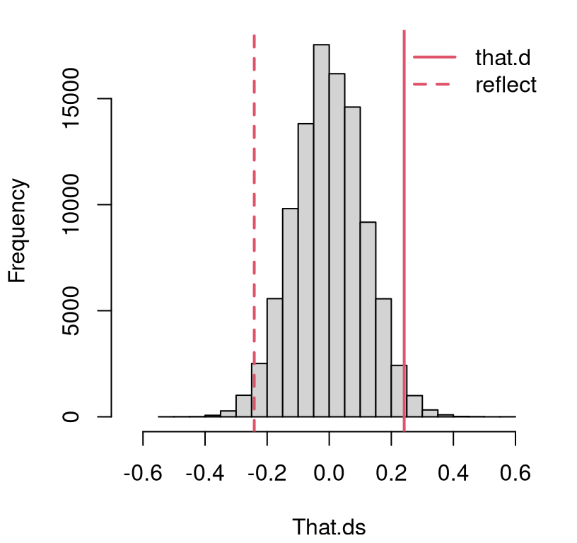

FIGURE 5.1: Histogram of sampled Bernoulli coin flip differences \(\hat{\theta}_\Delta = \hat{\theta}_y - \hat{\theta}_x\) compared to the value observed from data, and its reflection into the opposite tail.

This means that a \(p\)-value may be calculated by doubling the one-tailed calculation.

pval.mc <- 2*mean(That.ds >= that.d)
pval.mc

## [1] 0.0355

It’s a close call compared to the usual 5% threshold, but if we stick to that rule, then we would reject the null hypotheses and determine that \(\theta_y \ne \theta_x\). The coins that were flipped in the two campaigns were likely not the same.

Two-sample Bernoulli test by math

Recall that by either of the methods in Chapter 4, central limit theorem (CLT) or MLE, we have the following asymptotic approximations:

\[ \bar{Y} \equiv \hat{\theta}_y \sim \mathcal{N}(\theta_y, \theta_y(1 - \theta_y)/n_y) \quad \mbox{ and } \quad \bar{X} \equiv \hat{\theta}_x \sim \mathcal{N}(\theta_x, \theta_x(1 - \theta_x)/n_x) \]

as \(n_y \rightarrow \infty\) and \(n_x \rightarrow \infty\). Assuming independence between the samples and using (again) the trick that sums of Gaussians are Gaussian, we have

\[ \hat{\theta}_{\Delta} = \hat{\theta}_y - \hat{\theta}_x \sim \mathcal{N}\left(\theta_y - \theta_x, \frac{\theta_y(1 - \theta_y)}{n_y} + \frac{\theta_x(1 - \theta_x)}{n_x} \right) \quad \mbox{ as } \quad n_y, n_x \rightarrow \infty. \]

The null hypothesis, providing \(\theta \equiv \theta_y = \theta_x\), simplifies things substantially.

\[ \hat{\theta}_{\Delta} \sim \mathcal{N}\left(0, \theta(1 - \theta) \times \left(1/n_y + 1/n_x \right) \right) \quad \mbox{ as } \quad n_y, n_x \rightarrow \infty \]

Just like in §4.1, this result is of little use with unknown \(\theta\) in the variance, so it makes sense to replace it with an MLE. Remember, that’s legit because of the weak law of large numbers (WLLN). And we’re “Johnny on the spot” with \(\hat{\theta}_{\mathrm{pool}}\) from Eq. (5.4). This leads to a \(z\)-test after centering and scaling.

\[ Z = \frac{\hat{\theta}_y - \hat{\theta}_x}{ \sqrt{\hat{\theta}_{\mathrm{pool}}(1 - \hat{\theta}_{\mathrm{pool}}) \times \left(1/n_y + 1/n_x \right)}} \sim \mathcal{N}(0, 1) \quad \mbox{ as } \quad n_y, n_x \rightarrow \infty \]

Foregoing visuals, an approximate \(p\)-value may be calculated by following a familiar routine.

se <- sqrt(that.pool*(1 - that.pool)*(1/ny + 1/nx))
z <- that.d/se
pval.z <- 2*pnorm(-abs(z))
c(mc=pval.mc, z=pval.z)

##      mc       z 
## 0.03550 0.03345

That’s in pretty close agreement with our MC calculation, above. Both are approximations, but the difference is that one can always entertain bigger \(N\) to make a MC more accurate. With the CLT, \(n_x\) and \(n_y\) are what they are, far from infinity, and we’re stuck with that.

You may have wondered why I jumped straight to an asymptotic approximation. I did that because a closed-form distribution for \(\hat{\theta}_y - \hat{\theta}_x\), or any other related quantity, is not known. Approximations like this are all you’ll find in software. For example, in R the prop.test function provides a two-sample Bernoulli test.

pval.R <- prop.test(c(sx, sy), c(nx, ny), correct=FALSE)$p.value
pval.R

## [1] 0.03345

This is identical to pval.z above. I had to provide correct=FALSE to make it match what we calculated. According to R’s documentation, the default of correct=TRUE deploys a so-called Yates’ continuity correction. That page says “Yates’s correction should always be applied, as it will tend to improve the accuracy of the \(p\)-value obtained.” But this doesn’t feel right to me for two reasons. One is that the examples on that page are for contingency table tests for independence. This is related to our two-sample Bernoulli setting, but not identical. We’ll talk about that more in Chapter 10. The second reason is that the correction doesn’t make things better, on this example at least.

pval.Ry <- prop.test(c(sx, sy), c(nx, ny))$p.value
c(mc=pval.mc, z=pval.z, R=pval.R, Ry=pval.Ry)

##      mc       z       R      Ry 
## 0.03550 0.03345 0.03345 0.05785

One of these things is not like the others and leads to a different conclusion at the 5% level. Of course, any time you’re close to a threshold like 5%, whether that’s 3.3% or 5.8%, it probably makes sense to proceed with caution especially when approximations are involved. I like that I can just make \(N\) bigger and get a more accurate MC test.

---

Sometimes, textbooks will discuss how to build confidence intervals (CIs) for \(\theta_\Delta\). This is pretty straightforward, whether by MC or an asymptotic distribution. It’s of somewhat limited utility in my opinion, but it makes for a nice homework exercise. I suppose it can be helpful, in some instances, to provide an estimate (including uncertainties) of how far apart two population parameters could be.

5.2 Location

Now consider the same situation but with location models. Just to keep the running example going – don’t worry, we’re approaching the limits of its utility – consider again heights of women in my class. Instead of comparing to the population at large, suppose we compared to women on the Blacksburg High School (BHS) Women’s Varsity Basketball roster. Data on that page are converted to inches below.⁷

x <- c(5*12 + 6, 5*12 + 8, 5*12 + 6, 5*12 + 8, 6*12 + 2, 5*12 + 7, 
  5*12 + 10, 6*12 + 0, 5*12 + 7, 5*12 + 7)
nx <- length(x)
xbar <- mean(x)
s2x <- var(x)

As before, a vector y holds heights from my classroom (over-writing y for coin flips), but this is not printed to avoid duplication. Quantities ny, ybar and s2y are defined similarly. Figure 5.2 tries to help with a visual. Notice that there are two basketball players who are taller than the tallest woman from my class. Meanwhile, none are shorter than the shortest in my class. This is perhaps not surprising for a basketball team. However, that’s merely anecdotal as statistical analysis is concerned. The real question is if we have enough data to distinguish means, and how confident we are about that.

plot(y, abs(rnorm(ny, 0, 0.1)), ylim=c(-0.5, 2.25), 
  xlim=c(range(y, x)), xlab="heights", ylab="", yaxt="n", bty="n")
points(x, abs(rnorm(nx, 0.75, 0.1)), col=2, pch=19)
legend("top", c("class", "bball"), col=1:2, pch=c(21, 19), 
  bty="n", horiz=TRUE)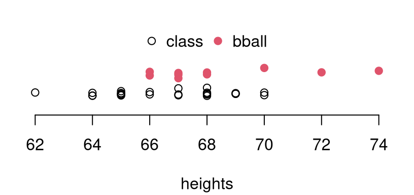

FIGURE 5.2: Comparing sample heights from my classroom and from the BHS basketball team. Vertical jitter is added to help visualize duplicate heights.

To get started on that “want to know”, it helps to be concrete about the modeling apparatus, which is the first step (it’s actually part of the “Assume”) in Alg. 1.1. We can’t get going without it.

\[\begin{align} \mbox{Model:} && Y_1, \dots, Y_{n_y} &\stackrel{\mathrm{iid}}{\sim} \mathcal{N}(\mu_y, \sigma_y^2) & & \mbox{and} & X_1, \dots, X_{n_x} &\stackrel{\mathrm{iid}}{\sim} \mathcal{N}(\mu_x, \sigma_x^2) \tag{5.5} \end{align}\]

You might wonder if Gaussians are appropriate for these data, especially for a basketball team where we might expect a distribution of heights that is not symmetric: a long right-hand tail and a stubby left one. That’s what Figure 5.2 shows. But, like in Chapter 2, let’s table that worry for now. I’ll get back to it later when I introduce nonparametric tests in Chapter 8. No modeling choice will be perfect. Gaussians are familiar, and they allow me to get on with explaining things.

Observe how this setup (5.5) is similar to Eq. (5.1) for coin flips, but with Gaussian location models. Hypotheses follow by analogy as well.

\[\begin{align} \mathcal{H}_0 &: \mu_y = \mu_x && \mbox{null hypothesis (``what if'')} \tag{5.6} \\ \mathcal{H}_1 &: \mu_y \ne \mu_x && \mbox{alternative hypothesis} \notag \end{align}\]

As in the single-Gaussian case (2.2), no specification is made for variances: \(\sigma_y^2\) and \(\sigma_x^2\). We could additionally presume they take on certain values, the same (unknown) value or different (unknown) values.

I’ll develop the latter two of those three cases, where the first one (an uncommon case) is akin to a simpler \(z\)-testing analog of the third, \(t\)-testing case. I shall privilege that one, since it’s the most common and likely the best suited to our situation, as pictured in Figure 5.2. The second one, known as the pooled variance case where \(\sigma^2 = \sigma_x^2 = \sigma_y^2\), is rather more niche. I believe it’s popular because of its rather simpler mathematical development. I’ll show you later. Via MC, however, the situation is reversed because the unpooled case is more compartmentalized: you basically just do two simulations like in §2.3 and combine them.

But I’m getting ahead of myself. MLE estimates (and bias-corrected variances) are straight out of §3.1. Let’s notate these as \(\hat{\mu}_y\), \(s_y^2\), \(\hat{\mu}_x\) and \(s_y^2\). No need to reiterate their formulation. Just treat \(y\)’s and \(x\)’s separately and run the numbers two times over. When pooling variance, first estimate means separately, and then combine the samples to assess uncertainty via Eq. (3.6).

\[\begin{equation} s^2_{\mathrm{pool}} = \frac{(n_y - 1) s_y^2 + (n_x - 1) s_x^2}{n_y + n_x - 2} = \frac{1}{n_y + n_x - 2} \left[ \sum_{i=1}^{n_y} (y_i - \bar{y})^2 + \sum_{i=1}^{n_x} (x_i - \bar{x})^2 \right] \tag{5.7} \end{equation}\]

So the pooled variance is a weighted average of individually calculated variances, with weights proportional to each sample size. Notice the \(-2\) in the denominator. This is important, correcting bias that arises from estimates of two quantities, \(\bar{Y}\) and \(\bar{X}\), costing two degrees of freedom (DoF).

np <- nx + ny
s2.pool <- ((ny - 1)*s2y + (nx - 1)*s2x)/(np - 2)

Before jumping in we need one more thing, a test statistic. Above in §5.1 for coin flips we looked at differences in averages. By analogy, that’s automatic here too. Again, the statistic is totally your choice as a practitioner, but it’s my job to nudge you in the right direction conceptually. One of the points of Chapter 4 is that statistics based on averages and MLEs (often also averages) are automatic because they have desirable properties. Let \(\mu_{\Delta} = \mu_y - \mu_x\), and under \(\mathcal{H}_0\) we have \(\mu_{\Delta} = 0\). A natural statistic for two-sample Gaussian testing is \(\hat{\mu}_{\Delta} = \hat{\mu}_y - \hat{\mu}_x = \bar{Y} - \bar{X}\).

muhat.d <- ybar - xbar

Two-sample Gaussian test by MC

First, the unpooled (\(\sigma_y^2 \ne \sigma_x^2\)) case. The code below follows the for loop in §2.3, augmented with \(\chi^2\) variances for \(t\)-tests from §3.2. Loop innards are duplicated to include both \(y\)- and \(x\)-calculations, saving differences in MLEs. You could do this without for loops, following exercise #10 from §3.5, but I don’t want to give that one away. The for loop way is a little slower, computationally, but more intuitive.

One caveat here is that, in order to respect \(\mathcal{H}_0\), the means of the two Gaussians must be the same (\(\mu = \mu_y = \mu_x\)). It actually doesn’t matter what value you use. My dad’s favorite baseball player was Mickey Mantle who wore #7 for the New York Yankees. So I’m going to use that: \(\mu = 7\). Try your favorite number and see what happens. If you had already sampled for one of the populations, say \(y\) from §3.2, then you could skip re-doing that as long as you used the same \(\mu\)-value as that simulation. I’m re-doing both samples below.

mu <- 7                                           ## RIP Dad and Mickey
Muhat.ds <- rep(NA, N)                   
for(i in 1:N) {  
  sigma2ys <- (ny - 1)*s2y/rchisq(1, ny - 1)      ## Y population (class)
  Ys <- rnorm(ny, mu, sqrt(sigma2ys))
  sigma2xs <- (nx - 1)*s2x/rchisq(1, nx - 1)      ## X population (bball)
  Xs <- rnorm(nx, mu, sqrt(sigma2xs)) 
  Muhat.ds[i] <- mean(Ys) - mean(Xs)              ## diff in averages           
}

Figure 5.3 provides a comparison between the empirical sampling distribution of differences in averages compared to the observed statistic. Just eyeballing it, I don’t think there’s enough evidence here to reject the null. The observed statistic \(\hat{\mu}_\Delta\), and its reflection, are partway into the tail(s), but not extreme relative to the sampling distribution.

hist(Muhat.ds, main="")
abline(v=c(muhat.d, -muhat.d), lty=1:2, col=2, lwd=2)
legend("topright", c("muhat.d", "reflect"), col=2, lty=1:2, lwd=2, bty="n")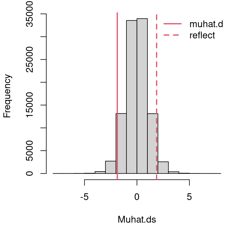

FIGURE 5.3: Histogram of sampled Gaussian average height differences \(\hat{\mu}_\Delta = \hat{\mu}_y - \hat{\mu}_x\) compared to the value observed from data, and its reflection into the opposite tail.

Here’s a more precise assessment through the lens of a \(p\)-value …

pval.mc <- 2*mean(Muhat.ds < muhat.d)
pval.mc

## [1] 0.0807

… indicating that there may not be enough evidence to reject \(\mathcal{H}_0\). We conclude that, although there are some tall women on the basketball team, those two samples could have come from (Gaussian) distributions with the same mean.

Code provided below goes back through the for loop implementing the pooled variance case.

Muhatp.ds <- rep(NA, N)                   
for(i in 1:N) {  
  sigma2s <- (np - 2)*s2.pool/rchisq(1, np - 2)   ## pooled variance
  Ys <- rnorm(ny, mu, sqrt(sigma2s))              ## Y sample (class)
  Xs <- rnorm(nx, mu, sqrt(sigma2s))              ## X sample (bball)
  Muhatp.ds[i] <- mean(Ys) - mean(Xs)             ## diff in averages           
}
pval.mcp <- 2*mean(Muhatp.ds < muhat.d)
pval.mcp

## [1] 0.03838

I’ve skipped the visual, but look what happens with the \(p\)-value. At the 5% level we would reject the null hypothesis, which is the opposite conclusion from earlier. So basically, what you decide comes down to a modeling choice. Pooling variances makes sense if you have a small amount of data, especially for one of the groups, and if you have reason to believe they’re similar. When that happens, you get a sharper sampling distribution that makes it easier to reject the null.

In our example, there are few women on the basketball team, \(n_x = 10\). Are variances similar? Looking at the spread of dots in Figure 5.2, perhaps they are. Both span about eight inches. But a choice about \(\sigma_x^2\) or \(\sigma_y^2\) is a modeling one. If you plan to use the data to help decide, then the right way to do that is via a statistical procedure that acknowledges sampling uncertainty. I plan to talk about that more in Chapter 6.

Two-sample Gaussian test by math

Quick digression. I know it’s awkward to digress before even getting started, and also not so quick. It turns out that what I thought was the gospel truth in two-sample Gaussian testing, known as the Welch test, is actually an approximation. The Welch test is what t.test in R does when you give it two samples, but it doesn’t warn you things might be off. Such betrayal! I would never have noticed if there wasn’t such a discrepancy between my MC calculation and the t.test output. I’ll show you in a moment; hold tight.

You’ll find the Welch test in every intro stats book, but I doubt you’ll find the straight story. Wikipedia gets it right. There’s really no better source for information in my opinion. You could make the case that this book is just a lens on Wikipedia focused on basic stats. Narrowing that focus on the two-sample Gaussian test, additional insight is provided by the page for the Behrens–Fisher (BF) problem, along with some citations to other approximate solutions.

The F in BF is for Ronald Fisher, the same Fisher as Fisher information from §4.2. Ronald is/was a super famous statistician, and geneticist, with a lot of statsy things named after him. He’s also a controversial figure. He picked a lot of fights with other scientists, and sometimes he was rude to them in print. Reading a Fisher paper is quite a trip. He had crazy ideas about racial issues and has been canceled by many modern progressive scientists as a result.

Fisher was good with numbers, and invented a whole field of statistics called fiducial inference, basically to address the two-sample Gaussian testing problem. He really went down a rabbit hole. My understanding is that the German chemist Walter-Ulrich Behrens solved the problem first (Behrens 1928), though perhaps less elegantly.

I’m not going to explain to you Behrens’ or Fisher’s solution, or fiducial inference. I don’t understand them. I did find an R package that will do the Behrens-Fisher test (Fay 2023). That implementation involves a numerical procedure, so it too provides an approximation of sorts. Importantly, it’s the kind of approximation that can be improved with better numerics (like MC, but unlike the CLT). I’m going to use that package to show you that it gives an answer closer to our MC result from above, than does the Welch test.

library(asht)
pval.bf <- bfTest(y, x)$p.value
pval.w <- t.test(y, x)$p.value
c(mc=pval.mc, bf=pval.bf, welch=pval.w)

##      mc      bf   welch 
## 0.08070 0.07676 0.06916

Notice how the MC and BF outcome rounds to the same hundredths place, but the Welch number does not. If you use \(10N\) MC simulations, then it will agree with BF to the one thousandths place. Considering how simple the MC approximation is, we can probably throw away the Welch test. Because it’s so common, I’m going to quickly explain it to you anyways.

Alright, back to what I intended to present before I got sidetracked. Welch (1938) showed that

\[ T = \frac{\bar{Y} - \bar{X}}{\sqrt{s_y^2/n_y + s_x^2/n_x}} \sim t_{\nu} \quad \mbox{ where } \quad \nu =\left\lfloor \frac{(s_y^2/n_y + s_x^2/n_x)^2}{ \frac{(s_y^2/n_y)^2}{n_y-1} + \frac{(s_x^2/n_x)^2}{n_x-1}} \right\rfloor, \]

approximately. The approximation improves as \(n_x, n_y \rightarrow \infty\), but that’s sort-of a moot point. Out at infinity you can just use a \(z\)-test via a CLT and not bother with that complicated DoF formula for \(\nu\). Wow, what a mouthful! That funny square bracket missing its top corners is the floor function, returning the largest integer smaller than its argument. This part is optional. The t.test function in R does not use the floor.

Here it goes in code.

se2 = s2y/ny + s2x/nx                     ## squared standard error
se <- sqrt(se2)                           ## standard error         
nu.denom <- (s2y/ny)^2/(ny - 1) + (s2x/nx)^2/(nx - 1)   
nu <- se2^2/nu.denom                      ## optionally nu <- floor(nu) 
t <- (ybar - xbar)/se                     ## t-stat
2*pt(-abs(t), nu)                         ## p-value

## [1] 0.06916

This agrees with pval.w above.

The pooled variance setup is simpler and less controversial, because getting it right mathematically is lots easier. You don’t have to invent a whole new way to think about uncertainty to get to the bottom of it. Since

\[ \sigma^2 \sim (n_y + n_x - 2) s^2_{\mathrm{pool}} / \chi^2_{n_y + n_x - 2}, \]

following a similar logic as in §3.2, a \(t\) statistic is readily available for testing.

\[\begin{equation} T = \frac{\bar{Y} - \bar{X}}{s_{\mathrm{pool}} \sqrt{1/n_y + 1/n_y}} \sim t_{n_x+n_y-2} \tag{5.8} \end{equation}\]

You’ll notice that this is the Gaussian-sample version of the pooled Bernoulli test above in §5.1. In code, along with the version from the t.test library function in R for comparison …

se.pool <- sqrt(s2.pool*(1/ny + 1/nx))
t <- (ybar - xbar)/se.pool
pval.tp <- 2*pt(-abs(t), ny + nx - 2)
c(mc=pval.mcp, math=pval.tp, lib=t.test(y, x, var.equal=TRUE)$p.value)

##      mc    math     lib 
## 0.03838 0.03833 0.03833

Everyone pretty much agrees.

---

As with the Bernoulli case, some textbooks and many software libraries provide CIs for \(\mu_\Delta\) along with tests. The t.test function does. I think it’s fairly basic, so I’ve left it to you as a homework exercise in §5.4. Remember, once you know the parameter estimate and standard error, which you do already once you have the sampling distribution for the test (3.11), there’s a simple adaptation to form a CI (3.20). If using MC simulation, just go back through the sim with estimated quantities (averages/MLEs) instead of values from \(\mathcal{H}_0\), which in this case means replacing 0.

5.3 Paired location

A special case that’s common when testing differences in means, whether for Gaussian populations or beyond, involves so-called paired data. This happens when experimental subjects in the \(y\)-group and \(x\)-group are linked together in some way as

\[ (x_1, y_1), (x_2, y_2), \dots, (x_n, y_n), \]

and consequently \(n \equiv n_x = n_y\). For example, suppose we asked each woman in my class (or, equivalently, each basketball player) to report their mother’s height when they were in college (or high school). Then we would have paired data. The result of a test on these paired data could be very interesting because it could tell us about the impact of socio-economic, behavioral, environmental and nutritional factors on health.

Quick digression on broader themes. There are many interesting questions you can ask about paired data. I bet correlation and prediction comes to mind, that is, using information about \(x\) to predict \(y\)? This is a very important topic, but not exactly what I’m intending to do here. We’ll get to that in Chapters 7 and 12. Here, I’m just considering two independent samples from related populations. It is the same setup as Eqs. (5.5) and (5.6), but different data collection environment.

Alright, back to what’s special about this paired setting. I asked the women in my class to provide their mother’s heights, and here are those values, below. I’m writing over the \(x\)’s from those basketball players. Their mothers’ heights aren’t available on the internet, unfortunately.

x <- c(64, 63, 68, 66, 67, 66, 66, 63, 66, 67, 69, 68, 70, 64, 68, 
  66, 65, 61, 69, 66, 61, 67, 63, 64)
nx <- length(x)

This time I’m not immediately jumping to parameter estimates for the two populations. There are two special, and cool, things about a paired test compared to the unpaired version. The first is that leveraging a paired structure eliminates some uncertainty, because there are fewer quantities to estimate. This gives you more power (§A.2) to reject the null. The second is that, when you’re doing it right, you reduce the problem to a simpler one that you already know how to solve, from Chapter 2, with some of the mathematical details in §3.2.

Before inference and testing, a good first step is visual. Figure 5.4 uses a scatterplot to inspect the mother-daughter relationship in the data. Mothers are on the \(x\)-axis and daughters on the \(y\)-axis, lining up with their variable names. Overlayed on the plot is a \(y=x\) line as an indication of parity in heights.

plot(x + rnorm(nx, sd=0.1), y + rnorm(ny, sd=0.1),  ## jitter for visual
  xlab="mothers (x)", ylab="daughters (y)") 
abline(0, 1)  ## intercept (a) = 0, slope (b) = 1 in y = ax + b. 
legend("bottomright", c("y = x"), lty=1)

FIGURE 5.4: Scatter plot showing mothers and daughters, with a \(y=x\) line overlayed for comparison.

If daughters tended to be the same heights as their mothers, then there would be about the same numbers of points above as below, with some lying exactly on the line in this case because data values are rounded to the nearest inch. Observe that there are more dots above the line than below (or on) the line. This suggests that these daughters are taller than their mothers. Is there enough evidence to reject the hippopotamus that they basically have the same mean height? That’s the “want to know”.

Assuming that \(x\)’s and \(y\)’s are uncorrelated – remember, we’ll get to the correlated case later – and that they are each Gaussian, their difference is also Gaussian:

\[ \mbox{Model:} \quad\quad D_i = Y_i - X_i \stackrel{\mathrm{iid}}{\sim} \mathcal{N}(\mu_d, \sigma_d^2), \quad\quad i=1, \dots, n. \]

If we’re willing to parameterize the individual populations (5.5), then we could work out \(\mu_d\) and \(\sigma_d^2\) in terms of those values using additivity of Gaussians, a trick that’s hopefully becoming familiar. But that is not our primary interest. If mothers and daughters have the same mean, then that means \(\mu_d = 0\), and so we have reduced our two-sample problem to a one-sample one.

d <- y - x
n <- length(d)
dbar <- mean(d)
s2d <- var(d)

Notice how only two quantities are being estimated, instead of four in §5.2. Now test …

\[\begin{align} \mathcal{H}_0 &: \mu_d = \textstyle 0 && \mbox{null hypothesis (``what if'')} \tag{5.9} \\ \mathcal{H}_1 &: \mu_d \ne 0 && \mbox{alternative hypothesis.} \notag \end{align}\]

Since this has been reduced to the one-sample case, I won’t show all variations. Let me encourage you to cut-and-paste the MC from §2.3. I’ll go straight for the math way from §3.2 along with a comparison to what the library provides in R.

se.d <- sqrt(s2d/n)
t.d <- dbar/se.d
pval.d <- 2*pt(-abs(t.d), n - 1)
c(math=pval.d, lib=t.test(y, x, paired=TRUE)$p.val)

##      math       lib 
## 0.0003117 0.0003117

Those are identical. The conclusion, with data from this particular example, is that daughters are indeed taller than their mothers. (An easy reject of \(\mathcal{H}_0\).)

You can similarly follow calculations from §3.3 to develop CIs if interested. No changes are required after reducing paired data \((x_i, y_i)\) to differences \(d_i = y_i - x_i\). In this case, the calculation is interesting, because it tells you how much taller daughters tend to be than their mothers.

q <- qt(c(0.025, 0.975), n - 1)
CI <- dbar + q*se.d
rbind(math=CI, lib=t.test(y, x, paired=TRUE)$conf.int)

##        [,1]  [,2]
## math 0.4691 1.364
## lib  0.4691 1.364

Again, our by-hand calculation and the R library agree. It looks like women in my class are between half-an-inch and 1.5 inches taller, very roughly speaking, than their mothers. Whether or not this is causal, and what the mechanism is, is a topic for another course.

5.4 Homework exercises

These exercises help gain experience with two-sample tests. Focus is on Bernoulli and Gaussian cases, as explained above, but there are some other unique settings too. My suggestion is to do each problem both ways: via MC and the math way (which might mean closed-form calculation or asymptotic approximation). Check with your instructor for details.

Do these problems with your own code, or code from this book. I encourage you to check your work with library functions like prop.test and t.test. Check with your instructor first to see what’s allowed. Unless stated explicitly otherwise, avoid use of libraries in your solutions.

#1: CI for \(\theta_\Delta\)

Develop code for MC and asymptotic approximations for a CI for \(\theta_\Delta\) in the two-sample Bernoulli setup of §5.1. Provide CI estimates for the coin-flipping example.

#2: Update monty.bern to include two-sample capabilities

Update monty.bern from §1.4, and possibly also §3.5 #6 and §4.4 #4, to include two-sample options. Follow these specifications.

• Make an optional x argument with x=NULL being the default, in which case one-sample versions (from earlier chapters) are used.
• Interpret theta as \(\theta_\Delta\) in this case.
• Support both MC and asymptotic approximations by checking N == -1.
• Optionally, augment with CI calculations for \(\theta_\Delta\) via #1, above.

Hint: the next three questions are pretty easy once you’ve done this one.

#3: Drone communication

A squadron of drones maintains a peer-to-peer communication protocol as they carry out maneuvers. Whenever a drone receives a signal from home base, it must relay the message to other members of the squadron following that protocol. A team is testing two different protocols, A and B, for their effectiveness while carrying out a schedule of prescribed maneuvers. Of the 198 Protocol-A messages sent from home base to the nearest drone, 169 of them were received by every drone in the squadron after one minute. Of the 155 Protocol-B messages sent to the nearest drone, 124 of them were received by every drone in the squadron after one minute. Do these protocols have the same success rate? Optionally, provide a CI for the difference in rates.

#4: Not in my back yard (NIMBY)

Blacksburg is a town in Montgomery county, Virginia. The county intends to green-light a new affordable housing project within town limits to alleviate a county-wide shortage. However, there’s concern that Blacksburg residents already have too many down-market developments, like those that cater to Virginia Tech students. A poll was taken to determine if there’s any difference between support for the project within town limits and in the broader county (excluding the town). Of the 209 townies who took the pool, 118 are in favor. Of the 488 county (non-Blacksburg) residents who took the pool, 211 are in favor. Is there any difference in voting patterns between the two groups. Optionally, provide a CI for the difference in voting rates.

#5: Truck pollution

In 2027 the US EPA will/has tighten(d) nitrogen oxide(s) (NOx) emission limits on diesel powered semi-trucks to 200 mg/bhp-hr. A major truck manufacturer has two models of these trucks, involving different diesel engines and NOx suppression technologies. In a sample of one-hundred trucks of both types, 16 of the first kind exceeded the threshold, while 12 of the second did. Is there any difference between the two models as concerns NOx emissions compliance? Optionally, provide the difference in rates exceeding the threshold.

#6: CI for \(\mu_{\Delta}\)

Develop code for MC and Welch approximations for a CI for \(\mu_\Delta\) in the two-sample Gaussian setup of §5.2, and also for \(\mu_d\) in the paired setup of §5.3. Provide CI estimates for women’s heights comparisons from those sections, studying differences between basketball players and mothers, respectively.

#7: Update monty.t to include two-sample capabilities

Update monty.t from §3.5 #8 to include two-sample options. Follow these specifications.

• Make an optional x argument with x=NULL being the default, in which case one-sample versions (from earlier) chapters are used.
• Interpret mu as \(\mu_\Delta\) in this case.
• Support both MC and Wald approximations by checking N == -1.
• Support a pooled=TRUE option (with FALSE being the default).
• Support a paired=TRUE option (with FALSE being the default), implementing a paired \(t\)-test. Note that pooled and paired don’t make sense at the same time. Be sure to check, in the paired case, that length(y) == length(x).
• Optionally, augment with CI calculations for \(\mu_{\Delta}\) and \(\mu_d\) via #6, above.

Hint: the next several questions are pretty easy once you’ve done this one.

#8: Physical therapy

Physical therapy (PT) is often recommended for patients recovering from surgery, but success can vary depending on many factors. In one study, two PT treatment centers were compared by measuring recovery time, in weeks, for knee replacement patients.

ptA <- c(38, 50, 41, 29, 45, 53, 46, 47, 39)
ptB <- c(61, 49, 50, 56, 58, 44, 65)

Is there a difference in mean recovery time for patients at the two PT centers? Optionally, provide a CI for the difference in mean recovery times.

#9: Dieting and weight loss

Twins who were interested in losing weight were recruited for a study of two different diets, paleo and keto, assigned to each sibling at random. The data below record the number of pounds (lbs) lost under each diet after six months. Each row corresponds to a pair of siblings.

paleo <- c(49, 6, 31, 14, 35, 31, 20, 64, 39)
keto <- c(25, 15, 17, 15, 33, 21, 32, 50, 14)
data.frame(paleo, keto)

##   paleo keto
## 1    49   25
## 2     6   15
## 3    31   17
## 4    14   15
## 5    35   33
## 6    31   21
## 7    20   32
## 8    64   50
## 9    39   14

Is there a difference in mean weight loss under the two diets? Optionally provide a CI for the difference in mean pounds lost.

#10: On the rocks

A bartender was curious about the shape of ice cubes in mixed drinks and performed an experiment. She wondered if one big ice cube was equivalent to several, small ice cubes of the same total volume, as affects the melting rate. (Melting rate is linked to both the temperature of the liquid in the cocktail, and how watered-down it tastes.) She filled identical tumblers with identical pours of room-temperature single-malt bourbon. One set of tumblers got a single one-inch cube of ice. The other got four half-inch cubes. She measured the amount of time (minutes) it took for all of the ice to dissolve, which is recorded below.

one <-  c(21.6, 20.1, 24.9, 18.8, 20.8, 25.2, 22.6, 28.3, 19.7, 28.7, 
    22.4, 14.8, 23.2, 21.6, 20.6)
four <- c(22.9, 17.2, 18.3, 21.2, 21.7, 23.4, 23.4, 17.4, 18.6, 18.3, 
    20.5, 21.4)

Is there is a difference in melting time for the different ice cubes? Does this change if we assume a pooled variance? Optionally, provide a CI for the difference in mean times.

#11: Return on investment

This is our first opportunity to really investigate the ROI claims from §2.5, which is available as roi.RData on the book webpage.

load("roi.RData")

Using roi$company and roi$industry, does there seem to be any difference in mean ROI between companies that use the IT product in question and the industry at large? Optionally, provide a confidence interval for the mean difference in ROI.

#12: Paired ROI

Data stored in roip.csv on the book webpage contains similar numbers, but company observations are paired, row-wise, with the industry observations that correspond to the ones they are associated with.

roip <- read.csv("roip.csv")

For example, Apple’s ROI is paired with the industry aggregate for high tech companies. This means that there are fewer unique roip$industry numbers, but roip$company is the same as roi$company. How does a paired analysis of these data compare with the unpaired one from #10?

#13: Simulation: lifetimes

We did two questions like this in §1.5. These next two are a little more complex because they involve two populations. For both, use simulations of size \(N=10^6\).

The lifetime of a major manufacturer’s name-brand LED light bulb in hours is \(Y \sim \mathrm{Exp}(\lambda = 10^{-4})\), and the generic, store-brand alternative is \(e^X\) where \(X \sim \mathcal{N}(\mu=6.5, \sigma^2=4.8)\), i.e., it’s log-normal. Answer the following.

1. What is the probability that the name-brand light bulb lasts longer than the generic, store-brand one?
2. What is the probability that it lasts two times longer?

#14: Simulation: intrusion kill chain

An intrusion kill chain is a model that is popular in some cybersecurity circles. The idea is based on a weakest link-in-the-chain concept. Suppose we were studying a kill chain with four links, and the amount of time available to detect and thwart a breach by disrupting an attack at any of the links is distributed as \(Y_i \sim \mathcal{N}(12, 2)\), for \(i=1,\dots,4\), in minutes. Note: 2 is the variance, so the standard deviation is \(\sqrt{2}\). One way to measure the robustness of a security system is to multiply the shortest time in the chain by the number of links. Call this the “kill time”.

1. Calculate the mean, median and standard deviation of the kill time.
2. To be considered robust enough for certain cybersecurity applications, the probability that the kill time is less than 30 minutes must be less than 0.01. Is this system robust enough?

#15: Poisson rate change

This one is challenging, but also fun.

The file changept.txt contains \(n=200\) samples that we can assume are independent Poisson. They are collected over time \(t=1, \dots, n\). In the parlance, the data comprise a time series.

y <- scan("changept.txt")

It is suspected that there is a change point \(m \in \{1,\dots,200\}\) somewhere along in time so that the first \(m\) observations are \(Y_t \stackrel{\mathrm{iid}}{\sim} \mathrm{Pois}(\theta)\), for \(t=1,\dots,m\), and the last \(n-m\) are \(X_t \stackrel{\mathrm{iid}}{\sim} \mathrm{Pois}(\phi)\), for \(t=m+1, \dots, n\).

1. Plot the data and guess \(\hat{m}\).
2. Using that \(\hat{m}\) argue that \(\theta \ne \phi\) via an appropriate statistical test that you design. Hint, no recipe is provided explicitly in this chapter, but you can combine ideas here with those in Chapters 3–4.
3. If you choose \(m\) differently – a little left or right, or a lot – how would your test from #b change?
4. How would you devise a statistical scheme to “dial in” a best \(m\) according to some well-defined statistical criteria?

References

Behrens, W. U. 1928. Ein Beitrag Zur Fehlerberechnung Bei Wenigen Beobachtungen. Institut für Pflanzenbau.

Fay, M. P. 2023. asht: Applied Statistical Hypothesis Tests. https://CRAN.R-project.org/package=asht.

Welch, B. L. 1938. “The Significance of the Difference Between Two Means When the Population Variances Are Unequal.” Biometrika 29 (3/4): 350–62. http://www.jstor.org/stable/2332010.

---

7. These data were accessed on April 10, 2025. If you access them at a different time, you will probably get different numbers. It might be interesting to additionally try with whatever you find.↩︎